How REML chooses smoothness#

A spline can follow the data as closely as you let it. The smoothing penalty decides how closely, and REML decides the penalty. This page says what that means, first in plain words, then in the maths, then in pictures on data where the true curve is known.

In plain words

A spline with forty pieces can copy the noise in the data as easily as the signal. The penalty charges the fit for wiggliness, and lambda is the price per unit of wiggle. REML sets the price by asking one question of the data: which amount of smoothness makes what we observed most probable, once the curve’s own uncertainty has been averaged out? No holdout set, no grid search; one criterion, maximised.

The maths#

The model is an additive predictor with one smooth per covariate:

\[ g(\mu_i) = \eta_i = \beta_0 + \sum_j f_j(x_{ij}), \qquad f_j(x) = \sum_{k=1}^{K_j} \beta_{jk}\, b_{jk}(x), \]

where the \(b_{jk}\) are basis functions (here B-splines) and \(K_j\) is the basis size, the k you pass to Spline. Fitting maximises a penalised log-likelihood,

\[ \ell_p(\boldsymbol\beta; \boldsymbol\lambda) = \ell(\boldsymbol\beta) - \tfrac{1}{2} \sum_j \lambda_j\, \boldsymbol\beta^\top \mathbf S_j\, \boldsymbol\beta , \]

in which \(\ell\) is the ordinary log-likelihood of the family and each \(\mathbf S_j\) is a penalty matrix measuring the wiggliness of \(f_j\). For a P-spline the penalty is the sum of squared second differences of neighbouring coefficients,

\[ \boldsymbol\beta^\top \mathbf S\, \boldsymbol\beta = \sum_{k=3}^{K} \left(\beta_k - 2\beta_{k-1} + \beta_{k-2}\right)^2 , \]

a discrete stand-in for \(\int f''(x)^2\,\mathrm{d}x\). A straight line has zero second differences, so the penalty cannot charge for one: lines are the penalty’s null space.

How much of the basis the fit actually uses is the effective degrees of freedom,

\[ \tau(\boldsymbol\lambda) = \operatorname{tr}(\mathbf F), \qquad \mathbf F = \left(\mathbf X^\top \mathbf W \mathbf X + \mathbf S_{\boldsymbol\lambda}\right)^{-1} \mathbf X^\top \mathbf W \mathbf X, \qquad \mathbf S_{\boldsymbol\lambda} = \sum_j \lambda_j \mathbf S_j , \]

where \(\mathbf X\) holds the basis functions evaluated at the data and \(\mathbf W\) the working weights of the fit. With \(\lambda = 0\) the trace is the rank of the identifiable design, one less than k here: the smooth is centred, so its constant direction belongs to the intercept and is constrained away, leaving 39 free degrees of freedom for a basis of 40. As \(\lambda \to \infty\) it falls to the size of the null space, one line’s worth. The EDF in every figure title below is this number.

REML chooses \(\boldsymbol\lambda\) by maximising the criterion Wood (2011) writes, for a fitted \(\hat{\boldsymbol\beta}\) at the given \(\boldsymbol\lambda\), as

\[ \mathcal V(\boldsymbol\lambda) = \ell(\hat{\boldsymbol\beta}) - \tfrac{1}{2}\hat{\boldsymbol\beta}^\top \mathbf S_{\boldsymbol\lambda}\hat{\boldsymbol\beta} + \tfrac{1}{2}\log\left|\mathbf S_{\boldsymbol\lambda}\right|_+ - \tfrac{1}{2}\log\left|\mathbf H + \mathbf S_{\boldsymbol\lambda}\right| + \tfrac{M_p}{2}\log(2\pi), \]

with \(\mathbf H\) the negative Hessian of \(\ell\) at \(\hat{\boldsymbol\beta}\) (for a GLM, \(\mathbf X^\top \mathbf W \mathbf X\)), \(|\cdot|_+\) the product of the non-zero eigenvalues, and \(M_p\) the dimension of the null space. For a Gaussian response this is exactly the restricted likelihood; for every other family it is the Laplace approximation to it, which is what fit_reml maximises.

Term

What it does

Why it matters

\(\ell(\hat{\boldsymbol\beta})\)

Rewards a fit that follows the data.

On its own it would always choose \(\lambda = 0\).

\(-\tfrac12 \hat{\boldsymbol\beta}^\top \mathbf S_{\boldsymbol\lambda} \hat{\boldsymbol\beta}\)

Charges the fitted curve for its wiggle at the current price.

The price is what is being chosen.

\(+\tfrac12 \log\lvert\mathbf S_{\boldsymbol\lambda}\rvert_+\)

Grows with \(\lambda\): the volume of curves the penalty considers plausible shrinks as the price rises.

This is the term that rewards simplicity.

\(-\tfrac12 \log\lvert\mathbf H + \mathbf S_{\boldsymbol\lambda}\rvert\)

Falls with \(\lambda\): the volume of curves the data leave plausible.

Together with the previous term it is the Occam factor: complexity is paid for automatically.

The Bayesian reading makes the balance intuitive. The penalty is a prior \(\boldsymbol\beta \sim N(\mathbf 0, \mathbf S_{\boldsymbol\lambda}^{-})\) that prefers smooth curves, and \(\mathcal V\) is the log probability of the data with the curve integrated out. Maximising it is asking which smoothness makes the observed data most probable.

Why REML and not a holdout#

Cross-validation needs many refits and a holdout that is not always available. Generalised cross-validation is a single criterion but Reiss and Ogden (2009) showed it has more local optima than REML and tends to under-smooth. Wood (2011) gave a stable Newton method for \(\mathcal V\) that also yields the smoothing-parameter uncertainty, and Wood, Pya and Säfken (2016) extended it to any regular likelihood. The holdout curve in the figures below is the check an actuary still trusts; on this data REML lands where it bottoms out.

Removing a term altogether#

The penalty cannot shrink its own null space, so an ordinary smooth can never disappear: at most it becomes a straight line. Marra and Wood (2011) add a second penalty on that null space, \(\lambda_j^{*} \mathbf S_j^{*}\) with \(\mathbf S_j^{*} = \mathbf U_j \mathbf U_j^\top\) built from the null-space eigenvectors of \(\mathbf S_j\), and let REML estimate both prices. That is select=True: a term with no signal can then be shrunk to zero, which the last figure shows.

What this means for a tariff

A curve that follows noise is a price that follows noise, and a price that follows noise is one a competitor can pick off. REML gives a reproducible, defensible choice of smoothness that a reviewer can read off the summary: the penalty, the effective degrees of freedom, and the criterion value at the optimum.

Words used above#

Word

Meaning here

Basis size, k

How many pieces the spline is built from; the most flexible the curve can be.

Penalty

A number that grows with the wiggliness of the curve.

Lambda

The price per unit of penalty; large means smooth.

EDF

Effective degrees of freedom: how many of the k pieces the fit really uses.

Null space

The shapes the penalty cannot charge for: straight lines.

REML

The criterion that chooses lambda from the data; for non-Gaussian families its Laplace approximation, sometimes written LAML.

Holdout deviance

The model’s error on rows it never saw; lower is better.

See it happen#

Four hundred points on a sine wave with a gentle slope, plus Gaussian noise with standard deviation 0.45. The basis is a P-spline with 40 functions, deliberately generous, so that an unpenalised fit has room to misbehave.

Hide code cell source

import numpy as np
import pandas as pd
from sklearn.model_selection import KFold

from superglm import Spline, SuperGLM, cross_validate

try:
    from myst_nb import glue
except ImportError:  # running outside the docs build, where nothing is glued

    def glue(name, obj, display=True):
        return obj


rng = np.random.default_rng(20260913)
n = 400
k = 40
noise_sd = 0.45
x = np.sort(rng.uniform(0.0, 1.0, n))
truth = np.sin(2 * np.pi * x) + 0.6 * x
y = truth + rng.normal(0.0, noise_sd, n)
X = pd.DataFrame({"x": x})
grid = pd.DataFrame({"x": np.linspace(0.0, 1.0, 300)})


def truth_on(frame):
    xs = frame["x"].to_numpy()
    return np.sin(2 * np.pi * xs) + 0.6 * xs

Move the price yourself#

Drag the slider and the left panel refits at that lambda; the right panel says how many effective degrees of freedom that price leaves. Run REML walks the optimiser’s own iterates, numbered, ending on the yellow tick, which is the lambda REML settled on.

Hide code cell source

import json

from IPython.display import HTML, display

SLIDER_TEMPLATE = """
<figure class="sg-slider" id="sg-slider-__NAME__">
  <div class="sg-slider__panels">
    <svg class="sg-slider__left" viewBox="0 0 640 300" role="img"
         aria-label="The spline fit at the selected lambda"></svg>
    <svg class="sg-slider__right" viewBox="0 0 640 300" role="img"
         aria-label="Effective degrees of freedom against lambda, with the REML iterates"></svg>
  </div>
  <div class="sg-slider__bar">
    <button type="button" class="sg-slider__btn sg-slider__sweep">Sweep</button>
    <button type="button" class="sg-slider__btn sg-slider__reml">Run REML</button>
    <input class="sg-slider__range" type="range" min="0" max="0" step="1" value="0"
           aria-label="lambda">
    <button type="button" class="sg-slider__btn sg-slider__jump">Jump to REML</button>
    <span class="sg-slider__readout"></span>
  </div>
  <noscript>Without JavaScript the slider does not run; the static figures below
  show the same fits at three fixed prices.</noscript>
</figure>
<script>
(function () {
  var D = __PAYLOAD__;
  var root = document.getElementById("sg-slider-__NAME__");
  if (!root) { return; }
  var NS = "http://www.w3.org/2000/svg";
  function el(tag, attrs, cls) {
    var node = document.createElementNS(NS, tag);
    for (var key in attrs) { node.setAttribute(key, String(attrs[key])); }
    if (cls) { node.setAttribute("class", cls); }
    return node;
  }
  function txt(svg, x, y, s, cls) {
    var node = el("text", {x: x, y: y}, cls);
    node.textContent = s;
    svg.appendChild(node);
    return node;
  }
  var T = 20, B = 258, L = 56, R = 624;
  var leftSvg = root.querySelector(".sg-slider__left");
  var rightSvg = root.querySelector(".sg-slider__right");
  var readout = root.querySelector(".sg-slider__readout");
  var range = root.querySelector(".sg-slider__range");
  var sweepBtn = root.querySelector(".sg-slider__sweep");
  var remlBtn = root.querySelector(".sg-slider__reml");
  var jumpBtn = root.querySelector(".sg-slider__jump");
  var P = D.path.lambdas;
  var n = D.lambdas.length;
  var current = 0;
  range.max = String(n - 1);

  var yAll = D.points[1].concat(D.truth);
  var ylo = Math.min.apply(null, yAll), yhi = Math.max.apply(null, yAll);
  var ypad = 0.08 * (yhi - ylo);
  ylo -= ypad; yhi += ypad;
  function fx(v) { return L + (R - L) * v; }
  function fy(v) { return B - (B - T) * (v - ylo) / (yhi - ylo); }
  function poly(xs, ys) {
    var out = [];
    for (var i = 0; i < xs.length; i++) {
      out.push(fx(xs[i]).toFixed(1) + "," + fy(ys[i]).toFixed(1));
    }
    return out.join(" ");
  }
  function fmt(v) {
    if (!(v > 0)) { return "0"; }
    if (v >= 1) { return v.toFixed(1); }
    return v.toExponential(1);
  }

  leftSvg.appendChild(el("line", {x1: L, y1: B, x2: R, y2: B}, "sg-slider__axis"));
  leftSvg.appendChild(el("line", {x1: L, y1: T, x2: L, y2: B}, "sg-slider__axis"));
  var dots = "";
  for (var i = 0; i < D.points[0].length; i++) {
    dots += "M" + fx(D.points[0][i]).toFixed(1) + " " + fy(D.points[1][i]).toFixed(1) + "h0";
  }
  leftSvg.appendChild(el("path", {d: dots}, "sg-slider__pt"));
  leftSvg.appendChild(el("polyline", {points: poly(D.x, D.truth)}, "sg-slider__truth"));
  var fitLine = el("polyline", {points: ""}, "sg-slider__fit");
  leftSvg.appendChild(fitLine);
  [0, 0.5, 1].forEach(function (v) {
    txt(leftSvg, fx(v) - 8, B + 18, String(v), "sg-slider__axis-label");
  });
  txt(leftSvg, R - 4, B + 18, "x", "sg-slider__axis-label");
  var leftTitle = txt(leftSvg, L, 14, "", "sg-slider__title");

  var emax = Math.max.apply(null, D.edf) * 1.12;
  var Z = 72, RL = 108;
  function rx(lam) {
    if (!(lam > 0)) { return Z; }
    var t = (Math.log(lam) / Math.LN10 + 4) / 8;
    return RL + (R - RL) * Math.max(0, Math.min(1, t));
  }
  function ry(v) { return B - (B - T) * v / emax; }
  rightSvg.appendChild(el("line", {x1: 40, y1: B, x2: R, y2: B}, "sg-slider__axis"));
  rightSvg.appendChild(el("line", {x1: 40, y1: T, x2: 40, y2: B}, "sg-slider__axis"));
  rightSvg.appendChild(el("line",
    {x1: rx(D.reml_lambda), y1: T, x2: rx(D.reml_lambda), y2: B}, "sg-slider__tick"));
  var gridPts = [];
  for (var i = 0; i < n; i++) {
    gridPts.push(rx(D.lambdas[i]).toFixed(1) + "," + ry(D.edf[i]).toFixed(1));
  }
  rightSvg.appendChild(el("polyline", {points: gridPts.join(" ")}, "sg-slider__grid"));
  var pathPts = [];
  for (var i = 0; i < P.length; i++) {
    pathPts.push(rx(P[i]).toFixed(1) + "," + ry(D.path.edf[i]).toFixed(1));
  }
  rightSvg.appendChild(el("polyline", {points: pathPts.join(" ")}, "sg-slider__path"));
  var iterDots = [];
  for (var i = 0; i < P.length; i++) {
    var c = el("circle", {cx: rx(P[i]).toFixed(1), cy: ry(D.path.edf[i]).toFixed(1), r: 5},
               "sg-slider__iter");
    rightSvg.appendChild(c);
    iterDots.push(c);
    txt(rightSvg, rx(P[i]) + 7, ry(D.path.edf[i]) - 7, String(i), "sg-slider__iternum");
  }
  var marker = el("circle", {cx: Z, cy: B, r: 5}, "sg-slider__marker");
  rightSvg.appendChild(marker);
  txt(rightSvg, Z - 12, B + 18, "0", "sg-slider__axis-label");
  [[-4, "1e-4"], [-2, "1e-2"], [0, "1"], [2, "1e2"], [4, "1e4"]].forEach(function (p) {
    txt(rightSvg, rx(Math.pow(10, p[0])) - 12, B + 18, p[1], "sg-slider__axis-label");
  });
  txt(rightSvg, 40, B + 34, "lambda (log scale, 0 at the left tick)", "sg-slider__axis-label");
  [0, Math.round(emax / 2), Math.round(emax / 1.12)].forEach(function (v) {
    txt(rightSvg, 8, ry(v) + 4, String(v), "sg-slider__axis-label");
  });
  txt(rightSvg, 40, 14, "EDF against lambda; red dots are REML's iterates",
      "sg-slider__title");

  function highlight(j) {
    for (var i = 0; i < iterDots.length; i++) {
      if (i === j) { iterDots[i].setAttribute("class", "sg-slider__iter sg-slider__iter--on"); }
      else { iterDots[i].setAttribute("class", "sg-slider__iter"); }
    }
  }
  function render(idx) {
    idx = Math.max(0, Math.min(n - 1, idx));
    current = idx;
    range.value = String(idx);
    fitLine.setAttribute("points", poly(D.x, D.curves[idx]));
    fitLine.setAttribute("class",
      idx === D.reml_index ? "sg-slider__fit sg-slider__fit--reml" : "sg-slider__fit");
    marker.setAttribute("cx", rx(D.lambdas[idx]).toFixed(1));
    marker.setAttribute("cy", ry(D.edf[idx]).toFixed(1));
    leftTitle.textContent = "fit at lambda = " + fmt(D.lambdas[idx]);
    readout.textContent = "\\u03bb = " + fmt(D.lambdas[idx]) + "   EDF " + D.edf[idx].toFixed(1);
  }
  function nearest(lam) {
    var best = 0, bd = Infinity, t = Math.log(Math.max(lam, 1e-12)) / Math.LN10;
    for (var i = 0; i < n; i++) {
      var d = Math.abs(Math.log(Math.max(D.lambdas[i], 1e-12)) / Math.LN10 - t);
      if (d < bd) { bd = d; best = i; }
    }
    return best;
  }

  var sweepTimer = null, remlTimer = null;
  function stopAll() {
    if (sweepTimer) { clearInterval(sweepTimer); sweepTimer = null; }
    if (remlTimer) { clearInterval(remlTimer); remlTimer = null; }
    sweepBtn.textContent = "Sweep";
    remlBtn.textContent = "Run REML";
  }
  sweepBtn.addEventListener("click", function () {
    if (sweepTimer) { stopAll(); return; }
    stopAll();
    sweepBtn.textContent = "Pause";
    var i = current >= n - 1 ? 0 : current;
    sweepTimer = setInterval(function () {
      i += 1;
      if (i >= n) { stopAll(); return; }
      render(i);
    }, 90);
  });
  remlBtn.addEventListener("click", function () {
    stopAll();
    remlBtn.textContent = "Running";
    var offset = P.length - D.path.objective.length;
    var j = -1;
    highlight(-1);
    remlTimer = setInterval(function () {
      j += 1;
      if (j >= P.length) { stopAll(); highlight(P.length - 1); return; }
      highlight(j);
      render(nearest(P[j]));
      var obj = D.path.objective[j - offset];
      readout.textContent = "iteration " + j + ": \\u03bb = " + fmt(P[j]) +
        ", EDF " + D.path.edf[j].toFixed(1) +
        (obj === undefined ? "" : ", objective " + obj);
    }, 700);
  });
  jumpBtn.addEventListener("click", function () { stopAll(); render(D.reml_index); });
  range.addEventListener("input", function () {
    stopAll();
    render(parseInt(range.value, 10));
  });
  render(0);
})();
</script>
"""


def slider_html(payload, name):
    return SLIDER_TEMPLATE.replace("__NAME__", name).replace(
        "__PAYLOAD__", json.dumps(payload)
    )


def fit_at(lam):
    model = SuperGLM(
        family="gaussian",
        spline_penalty=lam,
        features={"x": Spline(kind="ps", k=k)},
    )
    return model.fit(X, y)


reml = SuperGLM(
    family="gaussian",
    features={"x": Spline(kind="ps", k=k)},
).fit_reml(X, y)

lambdas = np.concatenate(([0.0], np.logspace(-4, 4, 60)))
curves, edfs = [], []
for lam in lambdas:
    swept = fit_at(lam)
    curves.append(np.round(swept.predict(grid), 3).tolist())
    edfs.append(round(float(swept.term_inference("x").edf), 2))

history = reml.reml_diagnostics()
reml_lambda = float(history["lambdas"]["x"])
reml_index = int(
    np.argmin(np.abs(np.log10(np.maximum(lambdas, 1e-12)) - np.log10(reml_lambda)))
)
path_lambdas = [float(step["x"]) for step in history["lambda_history"]]
path_edf = [round(float(fit_at(lam).term_inference("x").edf), 2) for lam in path_lambdas]
payload = {
    "x": np.round(grid["x"].to_numpy(), 4).tolist(),
    "truth": np.round(truth_on(grid), 3).tolist(),
    "points": [np.round(x, 4).tolist(), np.round(y, 3).tolist()],
    "lambdas": [float(v) for v in lambdas],
    "edf": edfs,
    "curves": curves,
    "reml_index": reml_index,
    "reml_lambda": reml_lambda,
    "path": {
        "lambdas": path_lambdas,
        "edf": path_edf,
        "objective": [round(float(v), 3) for v in history["objective_history"]],
    },
}
display(HTML(slider_html(payload, "reml")))

No penalty, REML, far too much penalty#

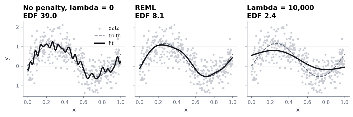
Three fits of the same model. The first fixes lambda at zero, the second lets fit_reml choose it, the third fixes it at ten thousand.

Hide code cell source

fits = [
    ("No penalty, lambda = 0", fit_at(0.0)),
    ("REML", reml),
    ("Lambda = 10,000", fit_at(1e4)),
]
for title, model in fits:
    print(f"{title:<24} EDF {model.term_inference('x').edf:5.1f}")
No penalty, lambda = 0   EDF  39.0
REML                     EDF   8.1
Lambda = 10,000          EDF   2.4
Hide code cell source

def draw(ax, title, model):
    ax.scatter(x, y, s=6, color="#C9CCD3", label="data", zorder=1)
    ax.plot(
        grid["x"], truth_on(grid),
        color="#6B7280", linestyle="--", linewidth=1.4, label="truth", zorder=2,
    )
    ax.plot(grid["x"], model.predict(grid), color="#15171C", linewidth=2.2, label="fit", zorder=3)
    edf = model.term_inference("x").edf
    ax.set_title(f"{title}\nEDF {edf:.1f}")
    ax.set_xlabel("x")


fig_three, axes = plt.subplots(1, 3, figsize=(9, 3.0), sharey=True)
for ax, (title, model) in zip(axes, fits):
    draw(ax, title, model)
axes[0].set_ylabel("y")
axes[0].legend(loc="upper right")
fig_three.tight_layout()
glue("lambda-triptych", fig_three, display=False)
Three fits of the same 400 points: no penalty, the REML penalty, and lambda ten thousand.

The same 400 points three times. With no penalty the spline chases every point. REML picks a penalty that follows the truth. A penalty far too large leaves the curve a slope and one gentle bend, and it misses the peaks.#

With no penalty the fit spends all 39 of its free degrees of freedom on the noise. With the REML lambda it spends about eight, and the curve sits on the truth. At lambda ten thousand it has two left, enough for a slope and a little bend, and misses the peaks entirely.

What the penalty buys#

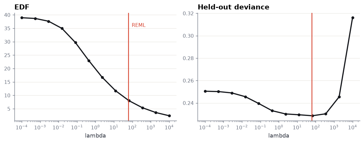
Now sweep lambda over a log grid of twelve fixed values and ask two things of each fit: how many effective degrees of freedom it keeps, and how well it predicts rows it did not see, measured by mean deviance over five folds.

Hide code cell source

lambdas = np.logspace(-4, 4, 12)
edf = []
holdout = []
for lam in lambdas:
    model = SuperGLM(
        family="gaussian",
        spline_penalty=lam,
        features={"x": Spline(kind="ps", k=k)},
    )
    edf.append(model.fit(X, y).term_inference("x").edf)
    cv = cross_validate(
        model, X, y,
        cv=KFold(5, shuffle=True, random_state=1),
        scoring=("deviance",),
    )
    holdout.append(cv.mean_scores["deviance"])

reml_lambda = reml.reml_diagnostics()["lambdas"]["x"]
print(f"REML chose lambda = {reml_lambda:.1f}")
REML chose lambda = 61.8

Hide code cell source

fig_sweep, axes = plt.subplots(1, 2, figsize=(9, 3.6))
for ax, values, label in zip(axes, (edf, holdout), ("EDF", "Held-out deviance")):
    ax.plot(lambdas, values, color="#15171C", marker="o", markersize=4)
    ax.axvline(reml_lambda, color="#D6402B", linewidth=1.4)
    ax.set_xscale("log")
    ax.set_xlabel("lambda")
    ax.set_title(label)
axes[0].text(
    reml_lambda * 1.5, max(edf) * 0.95, "REML", color="#D6402B", fontsize=9, va="top",
)
fig_sweep.tight_layout()
glue("edf-and-holdout", fig_sweep, display=False)
Effective degrees of freedom and held-out deviance against lambda on a log axis, with a red line at the lambda REML chose.

What the penalty buys. Left: how many effective parameters the spline keeps. Right: held-out deviance. The red line is the lambda REML chose without ever seeing a holdout.#

The left panel is the dial: each factor of ten in lambda takes away a few degrees of freedom. The right panel is the reason the dial matters. Held-out deviance is flat and high on the left, where every fit reproduces the noise, falls to a minimum, and rises steeply on the right, where the fits are too stiff to reach the peaks. REML never touched a fold and still landed at the bottom.

How REML gets there#

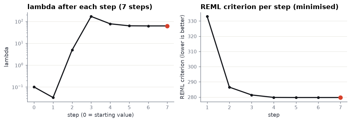
REML is an optimisation the solver drives directly, not a grid search. superglm minimises the negative REML criterion, so lower is better and the right-hand curve below falls. reml_diagnostics keeps the path the optimiser took: one lambda per outer step plus the starting value, and one criterion value per step.
Hide code cell source

diag = reml.reml_diagnostics()
path = [step["x"] for step in diag["lambda_history"]]
objective = list(diag["objective_history"])

fig_path, axes = plt.subplots(1, 2, figsize=(9, 3.2))
axes[0].plot(range(len(path)), path, color="#15171C", marker="o", markersize=4)
axes[0].plot(len(path) - 1, path[-1], color="#D6402B", marker="o", markersize=7)
axes[0].set_yscale("log")
axes[0].set_title(f"lambda after each step ({diag['n_reml_iter']} steps)")
axes[0].set_xlabel("step (0 = starting value)")
axes[0].set_ylabel("lambda")
axes[1].plot(range(1, len(objective) + 1), objective, color="#15171C", marker="o", markersize=4)
axes[1].plot(len(objective), objective[-1], color="#D6402B", marker="o", markersize=7)
axes[1].set_title("REML criterion per step (minimised)")
axes[1].set_xlabel("step")
axes[1].set_ylabel("REML criterion (lower is better)")
fig_path.tight_layout()
glue("reml-path", fig_path, display=False)
Two panels: lambda after each outer step on a log axis, and the REML criterion per step, both ending in a red marker.

REML is an optimisation the solver drives directly, not a grid search: a handful of steps from the starting value to the optimum on this example. Left, lambda after each step, where step 0 is the starting value, so the left panel carries one point more than the right. Right, the criterion superglm minimises, which is why the curve falls. In both panels the red marker is the value REML settled on.#

The path is not a steady climb. The optimiser probes downwards once, then climbs three orders of magnitude in two steps, overshoots, and settles back to a lambda near the bottom of the held-out curve in the previous figure. The criterion is within a fraction of a point of its final value after four steps; everything past that is refinement. A grid over twelve values, as in the previous figure, costs twelve fits and five folds each; the optimiser costs a handful of fits and no folds.

Removing a term that carries no signal#

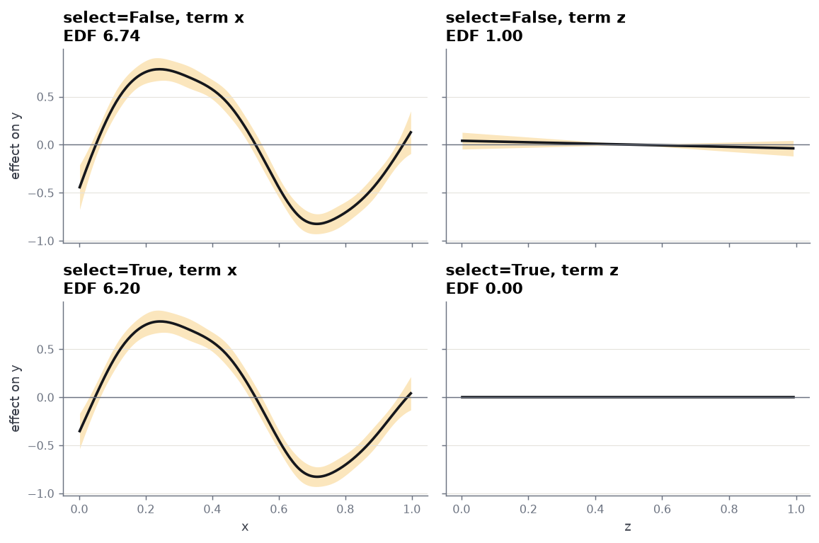
Add a second column z that has nothing to do with y, and fit both columns as splines. The ordinary penalty charges for bending, so a term it cannot justify is shrunk to a straight line, and a straight line costs nothing under that penalty, so it stays. select=True adds a second penalty on the straight part as well, and REML can then take the term out altogether.

Hide code cell source

z = rng.uniform(0.0, 1.0, n)
X2 = pd.DataFrame({"x": x, "z": z})

selected = {}
for sel in (False, True):
    selected[sel] = SuperGLM(
        family="gaussian",
        features={
            "x": Spline(kind="ps", k=12, select=sel),
            "z": Spline(kind="ps", k=12, select=sel),
        },
    ).fit_reml(X2, y)
    for name in ("x", "z"):
        print(f"select={sel!s:<5} {name}  EDF {selected[sel].term_inference(name).edf:6.3f}")
select=False x  EDF  6.745
select=False z  EDF  1.000
select=True  x  EDF  6.199
select=True  z  EDF  0.000
Hide code cell source

fig_select, axes = plt.subplots(2, 2, figsize=(9, 6), sharex="col", sharey=True)
for row, sel in enumerate((False, True)):
    for col, name in enumerate(("x", "z")):
        ax = axes[row, col]
        term = selected[sel].term_inference(name)
        # ci_lower and ci_upper are on the relativity scale; the curve is on the
        # linear-predictor scale, which for this Gaussian identity fit is the
        # effect on y. Take logs so the band and the curve share an axis.
        ax.fill_between(
            term.x, np.log(term.ci_lower), np.log(term.ci_upper),
            color="#F4B942", alpha=0.35, linewidth=0,
        )
        ax.plot(term.x, term.log_relativity, color="#15171C")
        ax.axhline(0.0, color="#6B7280", linewidth=0.8)
        ax.set_title(f"select={sel}, term {name}\nEDF {term.edf:.2f}")
        if row == 1:
            ax.set_xlabel(name)
        if col == 0:
            ax.set_ylabel("effect on y")
fig_select.tight_layout()
glue("select-shrinkage", fig_select, display=False)
A two-by-two grid of fitted effects with confidence bands: the x term and the z term, fitted with select off and on.

A term with no signal. The black curve is the fitted effect and the yellow band its 95% confidence interval. All four panels share one y axis, so the z term’s effect can be compared with the x term’s. Without the double penalty the z term keeps a slope and one degree of freedom, because the ordinary penalty cannot charge for a straight line; with select=True REML shrinks it to flat and its EDF to zero. The x term is untouched either way.#

References#

  • Wood, S. N. (2011). Fast stable restricted maximum likelihood and marginal likelihood estimation of semiparametric generalized linear models. Journal of the Royal Statistical Society: Series B, 73(1), 3–36. doi:10.1111/j.1467-9868.2010.00749.x

  • Wood, S. N., Pya, N., and Säfken, B. (2016). Smoothing parameter and model selection for general smooth models. Journal of the American Statistical Association, 111(516), 1548–1563. doi:10.1080/01621459.2016.1180986

  • Marra, G., and Wood, S. N. (2011). Practical variable selection for generalized additive models. Computational Statistics & Data Analysis, 55(7), 2372–2387. doi:10.1016/j.csda.2011.02.004

  • Reiss, P. T., and Ogden, R. T. (2009). Smoothing parameter selection for a class of semiparametric linear models. Journal of the Royal Statistical Society: Series B, 71(2), 505–523. doi:10.1111/j.1467-9868.2008.00695.x

  • Wood, S. N. (2017). Generalized Additive Models: An Introduction with R, 2nd edition. Chapman and Hall/CRC. doi:10.1201/9781315370279

  • Wahba, G. (1985). A comparison of GCV and GML for choosing the smoothing parameter in the generalized spline smoothing problem. Annals of Statistics, 13(4), 1378–1402. doi:10.1214/aos/1176349743

Main takeaways#

  • No penalty means the spline reproduces the noise; the effective degrees of freedom climb towards the basis size.

  • REML picks the penalty from the data alone, and on this example it lands where held-out deviance is lowest.

  • The optimiser reaches that value in a handful of steps; it is an optimisation the solver drives directly, not a grid search, and the criterion it drives down is the negative REML criterion, so lower is better.

  • select=True lets REML remove a term that carries no signal instead of leaving it a straight line.

Next steps#