
Smoothing Ordered Categorical Variables#
Insurance pricing data often arrives with continuous variables already binned into ordered categories — age bands, mileage bands, risk tiers. A plain categorical (one-hot) GLM estimates a free parameter per bin, which can be noisy. If we believe the underlying effect is smooth, we can exploit the ordering by fitting a spline on the numeric rank of the categories instead.
OrderedCategorical wraps this workflow: you pass the ordered labels, choose a
spline type, and get smoothed per-level relativities with SEs.
This notebook demonstrates:
OrderedCategorical— fit B-spline and cubic regression spline modelsRaw
Categorical— the unconstrained baseline for comparisonDiagnostic overlay — smoothed vs raw relativities on one plot
Boundary behaviour — how B-spline and cubic regression differ at the edges
We use the local French MTPL2 frequency parquet when available and fall back to
fetch_openml otherwise.
from pathlib import Path

import matplotlib.pyplot as plt
import numpy as np
import pandas as pd
from scipy.stats import norm

from superglm import Categorical, OrderedCategorical, Poisson, Spline, SuperGLM
from superglm.plotting.common import (
    _EXP_EDGE,
    _EXP_EDGE_LW,
    _EXP_FILL,
    _REF_COLOR,
    _REF_LW,
)

z = norm.ppf(0.975)
1. Data preparation#
We bin DrivAge into 18 ordered bands of 3–5 years each, simulating the
kind of pre-binned variable you’d receive from underwriting or a third-party
data provider.
from sklearn.datasets import fetch_openml

DATA_PATH = Path("../../data/freMTPL2freq.parquet")

if DATA_PATH.exists():
    df = pd.read_parquet(DATA_PATH)
else:
    df = fetch_openml(data_id=41214, as_frame=True, parser="auto").frame
df["ClaimNb"] = df["ClaimNb"].astype(float).clip(upper=4)
df["Exposure"] = df["Exposure"].astype(float).clip(lower=0.01)
df["DrivAge"] = df["DrivAge"].astype(float).clip(18, 90)

y = (df["ClaimNb"] / df["Exposure"]).to_numpy(dtype=float)
exposure = df["Exposure"].to_numpy(dtype=float)

# 18 ordered age bins (3-5 year width)
edges = [18, 21, 25, 29, 33, 37, 41, 45, 49, 53, 57, 61, 65, 69, 73, 77, 81, 85, 91]
labels = []
for i in range(len(edges) - 1):
    hi = edges[i + 1] - 1 if i < len(edges) - 2 else 90
    labels.append(f"{edges[i]}-{hi}")

n_levels = len(labels)

df["AgeBin"] = pd.cut(
    df["DrivAge"],
    bins=edges,
    labels=labels,
    right=False,
    include_lowest=True,
).astype(str)

print(f"{n_levels} bins from {labels[0]} to {labels[-1]}, {len(df):,} rows")
df[["DrivAge", "AgeBin"]].head(10)
18 bins from 18-20 to 85-90, 678,013 rows
| DrivAge | AgeBin | |
|---|---|---|
| 0 | 55.0 | 53-56 |
| 1 | 55.0 | 53-56 |
| 2 | 52.0 | 49-52 |
| 3 | 46.0 | 45-48 |
| 4 | 46.0 | 45-48 |
| 5 | 38.0 | 37-40 |
| 6 | 38.0 | 37-40 |
| 7 | 33.0 | 33-36 |
| 8 | 33.0 | 33-36 |
| 9 | 41.0 | 41-44 |
2. Three models#
We fit three Poisson GLMs on the same binned data:
Model |
Feature |
What it does |
|---|---|---|
B-spline |
|
Maps bins to 0–1 rank, fits a B-spline with 2nd-difference penalty |
Cubic regression |
|
Same rank mapping, but integrated f’’ penalty + f’’=0 at boundaries |
Raw OHE |
|
One free parameter per bin — the unconstrained baseline |
bs_k = 12  # equivalent to the former n_knots=8 B-spline configuration
cr_k = 10  # equivalent to the former n_knots=8 cubic-regression configuration

# B-spline
m_bs = SuperGLM(
    family=Poisson(),
    features={"AgeBin": OrderedCategorical(order=labels, basis=Spline(kind="bs", k=bs_k))},
    discrete=True,
)
m_bs.fit_reml(df[["AgeBin"]], y, sample_weight=exposure)
ti_bs = m_bs.term_inference("AgeBin")
print(f"B-spline:          edf = {ti_bs.edf:.1f}")

# Cubic regression spline
m_cr = SuperGLM(
    family=Poisson(),
    features={"AgeBin": OrderedCategorical(order=labels, basis=Spline(kind="cr", k=cr_k))},
    discrete=True,
)
m_cr.fit_reml(df[["AgeBin"]], y, sample_weight=exposure)
ti_cr = m_cr.term_inference("AgeBin")
print(f"Cubic regression:  edf = {ti_cr.edf:.1f}")

# Raw categorical (OHE)
m_ohe = SuperGLM(
    family=Poisson(),
    features={"AgeBin": Categorical(base="most_exposed")},
    discrete=True,
)
m_ohe.fit(df[["AgeBin"]], y, sample_weight=exposure)
ti_ohe = m_ohe.term_inference("AgeBin")
print(f"Raw categorical:   {len(ti_ohe.levels)} levels")
B-spline:          edf = 10.4
Cubic regression:  edf = 8.4
Raw categorical:   18 levels
3. Per-level relativities#
All three models produce per-level relativities through the same API.
OrderedCategorical returns kind="categorical" with smoothed values
at the K level positions.
rels_bs = m_bs.relativities(with_se=True)["AgeBin"]
rels_cr = m_cr.relativities(with_se=True)["AgeBin"]
rels_ohe = m_ohe.relativities(with_se=True)["AgeBin"]

print("B-spline relativities:")
rels_bs
B-spline relativities:
| level | relativity | log_relativity | se_log_relativity | |
|---|---|---|---|---|
| 0 | 18-20 | 2.348407 | 0.853737 | 0.038837 |
| 1 | 21-24 | 1.654949 | 0.503770 | 0.022517 |
| 2 | 25-28 | 1.090184 | 0.086346 | 0.016823 |
| 3 | 29-32 | 0.882318 | -0.125202 | 0.012081 |
| 4 | 33-36 | 0.836948 | -0.177994 | 0.013560 |
| 5 | 37-40 | 0.859850 | -0.150997 | 0.010520 |
| 6 | 41-44 | 0.932064 | -0.070354 | 0.012109 |
| 7 | 45-48 | 1.012728 | 0.012648 | 0.010811 |
| 8 | 49-52 | 1.000924 | 0.000923 | 0.011075 |
| 9 | 53-56 | 0.906786 | -0.097848 | 0.013047 |
| 10 | 57-60 | 0.855580 | -0.155975 | 0.013431 |
| 11 | 61-64 | 0.863531 | -0.146726 | 0.018761 |
| 12 | 65-68 | 0.877066 | -0.131173 | 0.017379 |
| 13 | 69-72 | 0.897285 | -0.108382 | 0.023020 |
| 14 | 73-76 | 0.948456 | -0.052920 | 0.022481 |
| 15 | 77-80 | 0.925340 | -0.077594 | 0.031512 |
| 16 | 81-84 | 0.786343 | -0.240362 | 0.050309 |
| 17 | 85-90 | 1.081236 | 0.078105 | 0.072282 |
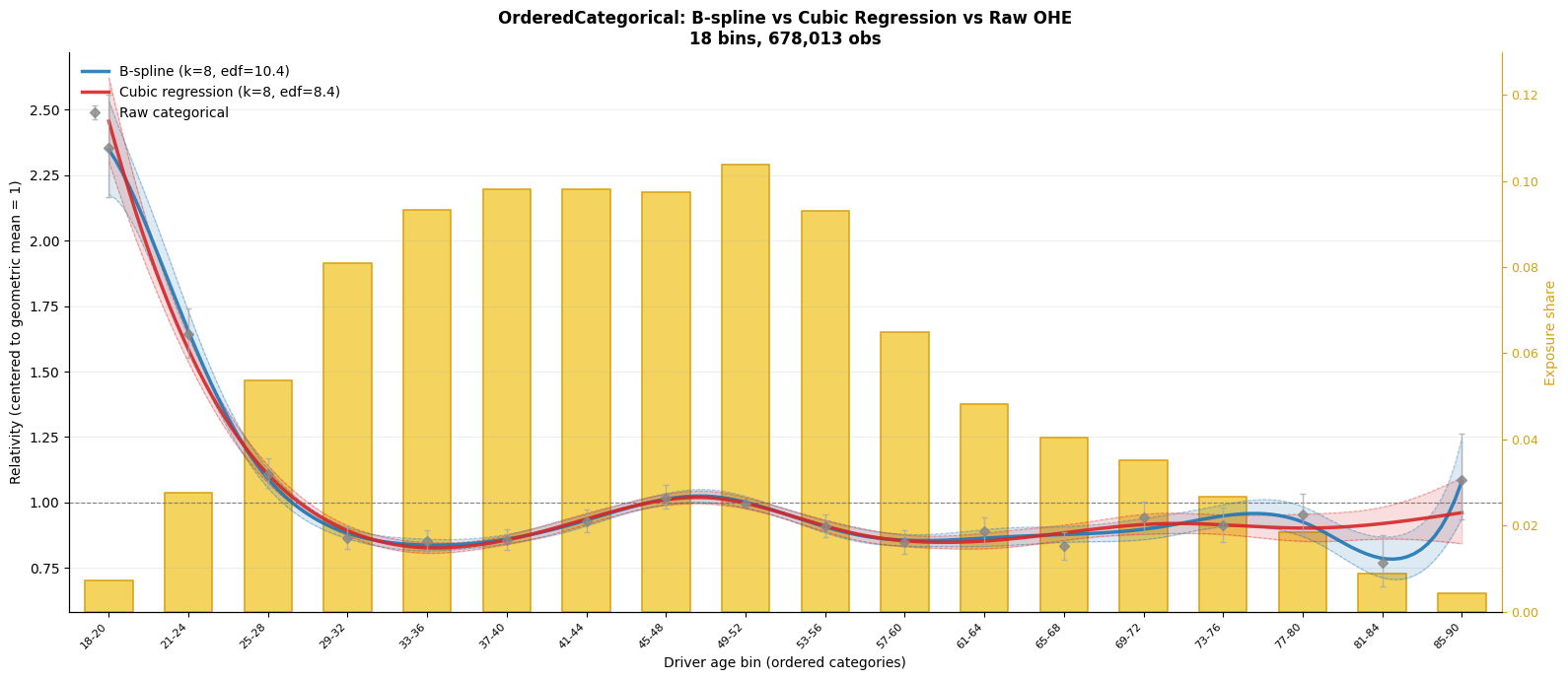
4. Diagnostic plot — smoothed vs raw#
To overlay spline and OHE relativities on the same axes, we re-center everything to geometric mean = 1 over the K levels. This is necessary because the spline uses sum-to-zero centering (SSP identifiability) while the categorical uses base-level centering — different reference points.
The re-centering is simple: exp(log_rel - mean(log_rel)) for each model,
applied consistently to both the level dots and the smooth curve.
# Exposure share per bin
exp_by_level = pd.DataFrame({"level": df["AgeBin"], "exp": exposure}).groupby("level")["exp"].sum()
exp_share = exp_by_level.reindex(labels, fill_value=0).values.copy()
exp_share /= exp_share.sum()

x_pos = np.arange(n_levels, dtype=float)

fig, ax = plt.subplots(figsize=(16, 7))

# Exposure bars
ax2 = ax.twinx()
ax2.bar(
    x_pos,
    exp_share,
    width=0.6,
    color=_EXP_FILL,
    edgecolor=_EXP_EDGE,
    linewidth=_EXP_EDGE_LW,
    alpha=1.0,
    zorder=0,
    label="Exposure share",
)
ax2.set_ylabel("Exposure share", color=_EXP_EDGE)
ax2.set_ylim(0, max(exp_share) * 1.25)
ax2.tick_params(axis="y", colors=_EXP_EDGE, labelsize=9)
ax2.spines["top"].set_visible(False)
ax2.spines["right"].set_color(_EXP_EDGE)
ax2.grid(False)
ax.set_zorder(ax2.get_zorder() + 1)
ax.patch.set_visible(False)

ax.axhline(1.0, color=_REF_COLOR, linewidth=_REF_LW, linestyle="--", zorder=0)


# Helper: plot smooth curve + CI, re-centered to geometric mean = 1
def plot_smooth(ax, ti, color, label):
    # Re-center: shift so geometric mean of level relativities = 1
    level_log_rels = np.asarray(ti.log_relativity, dtype=float)
    shift = level_log_rels.mean()

    curve = ti.smooth_curve
    x_fine = np.linspace(x_pos[0], x_pos[-1], len(curve.x))
    curve_rel = np.exp(np.asarray(curve.log_relativity, dtype=float) - shift)

    # CI band (also shifted)
    if curve.se_log_relativity is not None:
        se = np.asarray(curve.se_log_relativity, dtype=float)
        curve_log = np.asarray(curve.log_relativity, dtype=float) - shift
        ci_lo = np.exp(curve_log - z * se)
        ci_hi = np.exp(curve_log + z * se)
        ax.fill_between(x_fine, ci_lo, ci_hi, color=color, alpha=0.15, zorder=2)
        ax.plot(x_fine, ci_lo, color=color, linestyle="--", linewidth=0.7, alpha=0.4, zorder=3)
        ax.plot(x_fine, ci_hi, color=color, linestyle="--", linewidth=0.7, alpha=0.4, zorder=3)

    ax.plot(x_fine, curve_rel, color=color, linewidth=2.5, alpha=0.9, label=label, zorder=5)


plot_smooth(ax, ti_bs, "#1f77b4", f"B-spline (k={k}, edf={ti_bs.edf:.1f})")
plot_smooth(ax, ti_cr, "#d62728", f"Cubic regression (k={k}, edf={ti_cr.edf:.1f})")

# Raw OHE scatter with error bars (also re-centered to geometric mean = 1)
ohe_log_rels = np.asarray(ti_ohe.log_relativity, dtype=float)
ohe_shift = ohe_log_rels.mean()
ohe_rel = np.exp(ohe_log_rels - ohe_shift)
ohe_se = (
    np.asarray(ti_ohe.se_log_relativity, dtype=float)
    if ti_ohe.se_log_relativity is not None
    else None
)
if ohe_se is not None:
    ohe_ci_lo = np.exp((ohe_log_rels - ohe_shift) - z * ohe_se)
    ohe_ci_hi = np.exp((ohe_log_rels - ohe_shift) + z * ohe_se)
    yerr = [ohe_rel - ohe_ci_lo, ohe_ci_hi - ohe_rel]
else:
    yerr = None
ax.errorbar(
    x_pos,
    ohe_rel,
    yerr=yerr,
    fmt="D",
    color="#888888",
    markersize=5,
    alpha=0.8,
    ecolor="#aaaaaa",
    elinewidth=1.0,
    capsize=2,
    label="Raw categorical",
    zorder=6,
)

ax.set_xticks(x_pos)
ax.set_xticklabels(labels, rotation=45, ha="right", fontsize=8)
ax.set_xlim(-0.5, n_levels - 0.5)
ax.set_xlabel("Driver age bin (ordered categories)")
ax.set_ylabel("Relativity (centered to geometric mean = 1)")
ax.set_title(
    f"OrderedCategorical: B-spline vs Cubic Regression vs Raw OHE\n"
    f"{n_levels} bins, {len(df):,} obs",
    fontweight="bold",
)
ax.grid(alpha=0.22, axis="y")
ax.spines["top"].set_visible(False)
ax.spines["right"].set_visible(False)
ax.legend(frameon=False, loc="upper left")
fig.tight_layout()
plt.show()
5. Key takeaways#
Raw Categorical |
OrderedCategorical (spline) |
|
|---|---|---|
Parameters |
K-1 free |
~edf (REML-selected) |
Assumption |
None — each bin independent |
Smooth underlying effect |
Noisy tails |
Wide CIs, erratic |
Borrows strength from neighbours |
Boundary |
N/A |
|
Use case |
Unordered categories (region, vehicle type) |
Ordered/binned continuous variables |
The spline doesn’t change the model — it changes the parameterisation. Instead of K-1 free parameters, you get a smooth curve controlled by a penalty, with REML choosing how much to smooth. The raw OHE estimates serve as a diagnostic: if the spline diverges substantially from the OHE dots, the smoothness assumption may not hold.