SuperGLM Plotting Utilities — Full Inspection

Comprehensive review of all plotting and diagnostic utilities on the full French MTPL2 frequency dataset (678k rows). Everything Plotly-based where available, matplotlib fallback where not.

Sections:

1. Data prep & model fit

2. Main effects — Plotly explorer

3. Interaction plots — surface, contour, contour+HDR

4. Residual diagnostics (4-panel)

5. Residual type comparison

6. Lift chart

7. Double lift chart

8. Lorenz curve + Gini

9. Loss ratio chart

10. Term importance

import time
from pathlib import Path

import matplotlib.pyplot as plt
import numpy as np
import pandas as pd
import plotly.graph_objects as go
import plotly.io as pio
import plotly.subplots as sp
from scipy import stats

pio.renderers.default = "notebook_connected"  # noqa: E402

from superglm import Categorical, Poisson, Spline, SuperGLM  # noqa: E402
from superglm.diagnostics import term_importance  # noqa: E402
from superglm.validation import (  # noqa: E402
    double_lift_chart,
    lift_chart,
    lorenz_curve,
    loss_ratio_chart,
)

1. Data prep & model fit

t0 = time.perf_counter()

DATA_PATH = Path("../../data/freMTPL2freq.parquet")

if DATA_PATH.exists():
    df = pd.read_parquet(DATA_PATH)
else:
    from sklearn.datasets import fetch_openml

    df = fetch_openml(data_id=41214, as_frame=True, parser="auto").frame

# Standard cleaning
df["ClaimNb"] = df["ClaimNb"].astype(float).clip(upper=4)
df["Exposure"] = df["Exposure"].astype(float).clip(lower=0.01)
df["DrivAge"] = df["DrivAge"].astype(float).clip(18, 90)
df["VehAge"] = df["VehAge"].astype(float).clip(0, 20)
df["BonusMalus"] = df["BonusMalus"].astype(float).clip(50, 150)
df["Density"] = df["Density"].astype(float)
df["VehPower"] = df["VehPower"].astype(float)
df["LogDensity"] = np.log1p(df["Density"])

y = (df["ClaimNb"] / df["Exposure"]).to_numpy(dtype=np.float64)
exposure = df["Exposure"].to_numpy(dtype=np.float64)

features_to_use = ["DrivAge", "VehAge", "BonusMalus", "LogDensity", "Area", "VehPower"]
X = df[features_to_use].copy()

print(f"Rows: {len(df):,}")
print(f"Claim frequency: {df['ClaimNb'].sum() / df['Exposure'].sum():.4f}")
print(f"Zero-claim fraction: {(df['ClaimNb'] == 0).mean():.1%}")
print(f"[{time.perf_counter() - t0:.2f}s]")

Rows: 678,013
Claim frequency: 0.1006
Zero-claim fraction: 95.0%
[0.12s]

model = SuperGLM(
    family=Poisson(),
    selection_penalty=0,
    discrete=True,
    features={
        "DrivAge": Spline(n_knots=10, penalty="ssp"),
        "VehAge": Spline(n_knots=8, penalty="ssp"),
        "BonusMalus": Spline(n_knots=8, penalty="ssp"),
        "LogDensity": Spline(n_knots=7, penalty="ssp"),
        "Area": Categorical(base="first"),
        "VehPower": Spline(n_knots=7, penalty="ssp"),
    },
    interactions=[("DrivAge", "VehAge")],
)

t0 = time.perf_counter()
model.fit_reml(X, y, sample_weight=exposure, max_reml_iter=6)
print(f"Full model fit: {time.perf_counter() - t0:.1f}s")

mu = model.predict(X)
print(f"Mean predicted frequency: {np.average(mu, weights=exposure):.4f}")
print(f"Mean observed frequency:  {np.average(y, weights=exposure):.4f}")

model.summary()

Full model fit: 4.0s
Mean predicted frequency: 0.1006
Mean observed frequency:  0.1006

SuperGLM Results
Family:	Poisson		No. Observations:	678013
Link:	Log		Df (effective):	64.18 (39.51 smooth)
Method:	REML, discrete		Penalty:	None
Scale (phi):	1.000		Pearson chi2:	1410069.5
Log-Likelihood:	-130663.1		AIC:	261454.6
AICc:	261454.6		BIC:	262188.0
EBIC:	262188.0		Converged:	True (6 iter)
Deviance:	211532.1
	coef	std err	z	P>|z|	[0.025	0.975]	Sig	QS
Intercept	-2.3609	0.0382	-61.855	0.000	-2.436	-2.286	***
DrivAge
DrivAge	[spline, 13 params, χ²(10.4)=1019.6, p=<0.001] rank=13, edf=9.3, λ=12, curve SE: 0.01–0.10							***
▶ coefficient detail # coef std err z P>|z| [ci_lo ci_hi] Sig QS 1 0.0589 0.0845 0.697 0.485 -0.107 0.225 2 -0.0924 0.0452 -2.044 0.041 -0.181 -0.004 * 3 -0.1818 0.0303 -6.005 0.000 -0.241 -0.122 *** 4 -0.1818 0.0282 -6.445 0.000 -0.237 -0.126 *** 5 -0.0737 0.0290 -2.541 0.011 -0.131 -0.017 * 6 0.0901 0.0337 2.673 0.008 0.024 0.156 ** 7 -0.0707 0.0357 -1.980 0.048 -0.141 -0.001 * 8 -0.0515 0.0395 -1.304 0.192 -0.129 0.026 9 -0.0301 0.0450 -0.669 0.504 -0.118 0.058 10 0.0592 0.0538 1.099 0.272 -0.046 0.165 11 -0.0167 0.0662 -0.253 0.800 -0.146 0.113 12 0.0246 0.0687 0.359 0.720 -0.110 0.159 13 0.0334 0.0243 1.378 0.168 -0.014 0.081
VehAge
VehAge	[spline, 11 params, χ²(10.9)=6985.6, p=<0.001] rank=11, edf=10.8, λ=0.065, curve SE: 0.01–0.07							***
▶ coefficient detail # coef std err z P>|z| [ci_lo ci_hi] Sig QS 1 -3.3564 0.1494 -22.459 0.000 -3.649 -3.064 *** 2 -0.6690 0.0348 -19.211 0.000 -0.737 -0.601 *** 3 -0.5290 0.0443 -11.948 0.000 -0.616 -0.442 *** 4 -0.1511 0.0376 -4.015 0.000 -0.225 -0.077 *** 5 -0.6056 0.0465 -13.037 0.000 -0.697 -0.515 *** 6 -0.4887 0.0478 -10.229 0.000 -0.582 -0.395 *** 7 -0.7181 0.0694 -10.347 0.000 -0.854 -0.582 *** 8 -0.8036 0.1032 -7.786 0.000 -1.006 -0.601 *** 9 0.4114 0.3208 1.282 0.200 -0.217 1.040 10 -1.0663 0.3132 -3.404 0.001 -1.680 -0.452 *** 11 0.1884 0.1143 1.649 0.099 -0.036 0.412 .
BonusMalus
BonusMalus	[spline, 11 params, χ²(10.1)=5402.1, p=<0.001] rank=11, edf=9.7, λ=0.49, curve SE: 0.01–0.13							***
▶ coefficient detail # coef std err z P>|z| [ci_lo ci_hi] Sig QS 1 -0.5356 0.1603 -3.342 0.001 -0.850 -0.221 *** 2 0.4395 0.0381 11.532 0.000 0.365 0.514 *** 3 -0.1032 0.0545 -1.892 0.058 -0.210 0.004 . 4 0.4954 0.0552 8.973 0.000 0.387 0.604 *** 5 -0.4671 0.0705 -6.625 0.000 -0.605 -0.329 *** 6 0.6951 0.0884 7.860 0.000 0.522 0.868 *** 7 -0.3562 0.1212 -2.940 0.003 -0.594 -0.119 ** 8 0.5874 0.1769 3.320 0.001 0.241 0.934 *** 9 -0.0436 0.3421 -0.127 0.899 -0.714 0.627 10 0.0214 0.2583 0.083 0.934 -0.485 0.528 11 0.0972 0.0394 2.467 0.014 0.020 0.174 *
LogDensity
LogDensity	[spline, 10 params, χ²(1.1)=5.6, p=0.017] rank=10, edf=1.2, λ=1.3e+04, curve SE: 0.01–0.07							*
▶ coefficient detail # coef std err z P>|z| [ci_lo ci_hi] Sig QS 1 -0.0003 0.0027 -0.092 0.927 -0.006 0.005 2 -0.0059 0.0035 -1.655 0.098 -0.013 0.001 . 3 -0.0211 0.0087 -2.435 0.015 -0.038 -0.004 * 4 -0.0281 0.0115 -2.433 0.015 -0.051 -0.005 * 5 -0.0236 0.0100 -2.359 0.018 -0.043 -0.004 * 6 -0.0102 0.0055 -1.861 0.063 -0.021 0.001 . 7 0.0002 0.0034 0.049 0.961 -0.007 0.007 8 0.0212 0.0087 2.449 0.014 0.004 0.038 * 9 0.0265 0.0111 2.390 0.017 0.005 0.048 * 10 0.0192 0.0091 2.104 0.035 0.001 0.037 *
Area
Area[B]	0.0130	0.0260	0.498	0.619	-0.038	0.064
Area[C]	0.0055	0.0342	0.160	0.873	-0.062	0.072
Area[D]	0.0342	0.0509	0.673	0.501	-0.065	0.134
Area[E]	0.0354	0.0670	0.528	0.597	-0.096	0.167
Area[F]	-0.0237	0.0920	-0.258	0.796	-0.204	0.157
VehPower
VehPower	[spline, 10 params, χ²(9.0)=271.5, p=<0.001] rank=10, edf=8.5, λ=1.2, curve SE: 0.01–0.09							***
▶ coefficient detail # coef std err z P>|z| [ci_lo ci_hi] Sig QS 1 0.3457 0.1426 2.425 0.015 0.066 0.625 * 2 -0.0739 0.0348 -2.123 0.034 -0.142 -0.006 * 3 0.4967 0.0654 7.600 0.000 0.369 0.625 *** 4 -0.3300 0.0463 -7.127 0.000 -0.421 -0.239 *** 5 0.3660 0.0673 5.440 0.000 0.234 0.498 *** 6 0.0366 0.0834 0.439 0.661 -0.127 0.200 7 -0.0893 0.1139 -0.784 0.433 -0.312 0.134 8 -0.0346 0.2108 -0.164 0.870 -0.448 0.378 9 0.1266 0.1821 0.695 0.487 -0.230 0.483 10 -0.0497 0.0444 -1.119 0.263 -0.137 0.037
DrivAge:VehAge
DrivAge:VehAge	-0.0136	0.0537	-0.253	0.801	-0.119	0.092
Signif. codes: 0 '***' 0.001 '**' 0.01 '*' 0.05 '.' 0.1 ' ' 1
Note: smooth p-values use Wood (2013) Bayesian test. Parametric p-values are Wald approximations. For borderline significance, use a likelihood ratio test.

2. Main effects — Plotly explorer

Interactive multi-term explorer with term dropdown, response/link scale toggle, density overlays, knot markers, and CI bands.

t0 = time.perf_counter()
fig = model.plot(
    engine="plotly",
    X=X,
    sample_weight=exposure,
    ci="pointwise",
    show_knots=True,
)
fig.update_layout(height=550, title_text="Main Effects Explorer")
fig.show()
print(f"[{time.perf_counter() - t0:.2f}s]")

[10.35s]

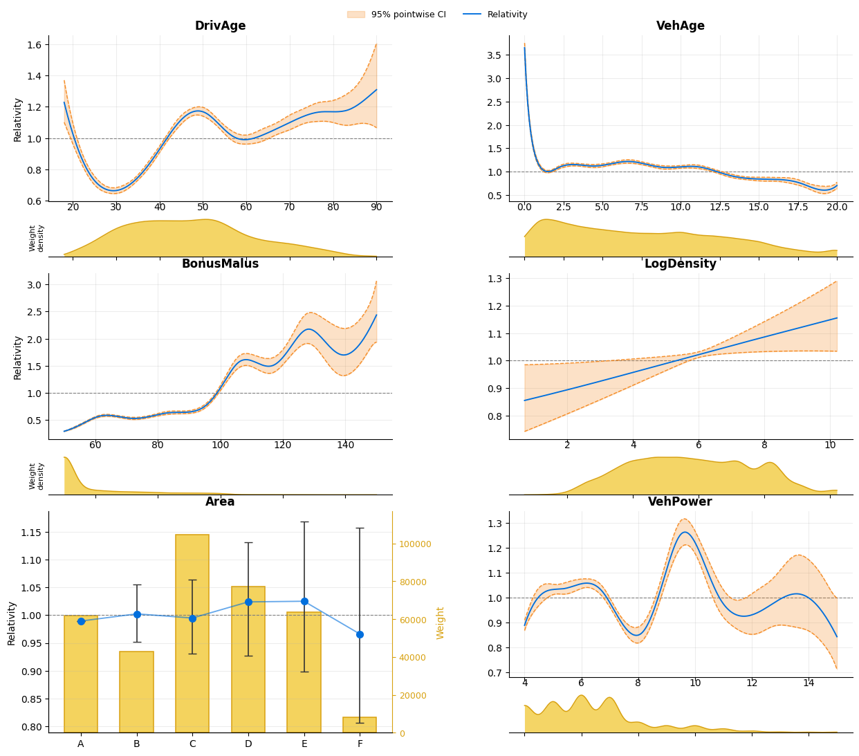
2b. Static matplotlib grid (for comparison)

t0 = time.perf_counter()
fig = model.plot(X=X, sample_weight=exposure, figsize=(15, 12))
fig.subplots_adjust(wspace=0.34, hspace=0.24)
plt.show()
print(f"[{time.perf_counter() - t0:.2f}s]")

[10.76s]

3. Interaction plots

3a. 3D surface

t0 = time.perf_counter()
fig = model.plot(
    "DrivAge:VehAge",
    engine="plotly",
    interaction_view="surface",
    X=X,
    sample_weight=exposure,
    n_points=200,
)
fig.update_layout(height=600, title_text="DrivAge:VehAge Interaction Surface")
fig.show()
print(f"[{time.perf_counter() - t0:.2f}s]")

[4.02s]

3b. Contour view

t0 = time.perf_counter()
fig = model.plot(
    "DrivAge:VehAge",
    engine="plotly",
    interaction_view="contour",
    X=X,
    sample_weight=exposure,
    n_points=200,
)
fig.update_layout(height=500, title_text="DrivAge:VehAge Contour")
fig.show()
print(f"[{time.perf_counter() - t0:.2f}s]")

[0.03s]

3c. Contour pair with exposure HDR density

t0 = time.perf_counter()
fig = model.plot(
    "DrivAge:VehAge",
    engine="plotly",
    interaction_view="contour_pair",
    X=X,
    sample_weight=exposure,
    n_points=220,
)
fig.update_layout(height=500, title_text="Interaction Effect + Exposure Density")
fig.show()
print(f"[{time.perf_counter() - t0:.2f}s]")

[4.51s]

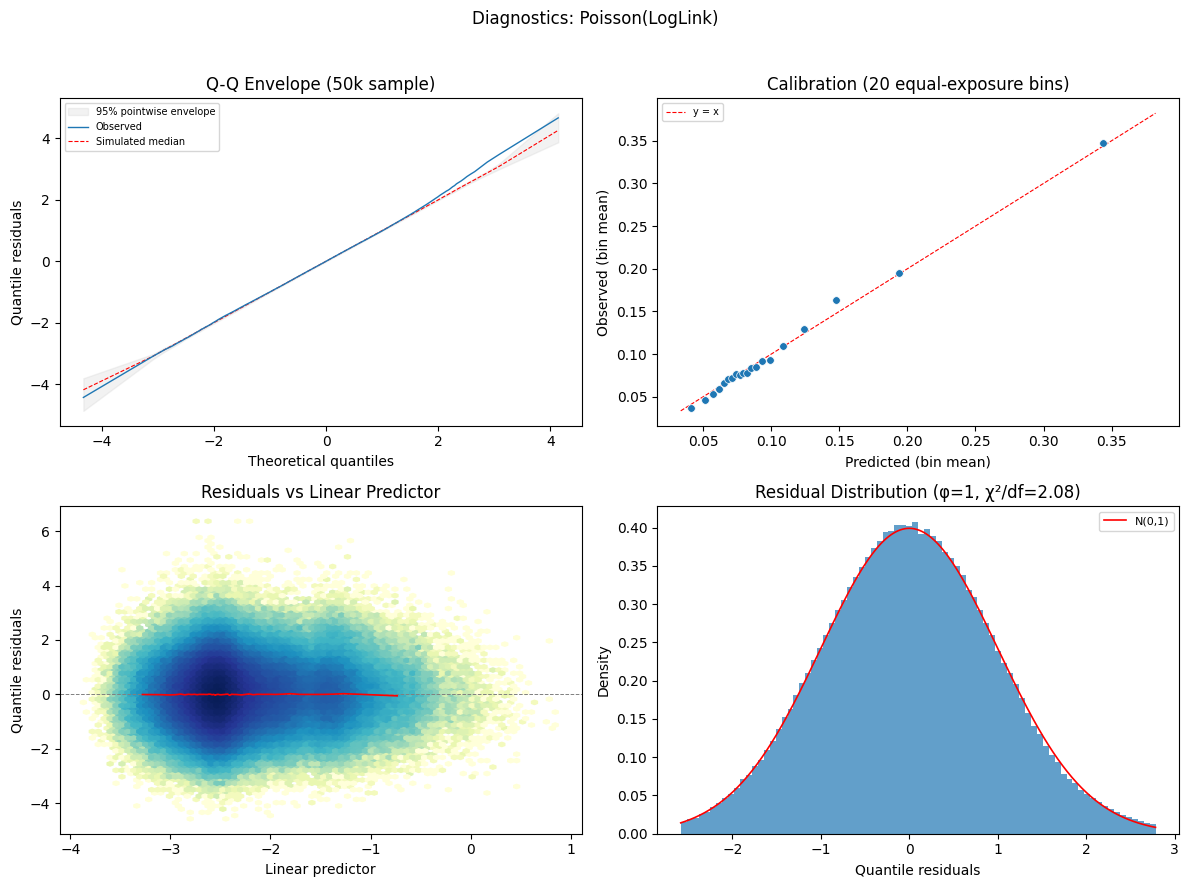
4. Residual diagnostics — GLM/GAM style

Four panels using quantile residuals (Dunn & Smyth 1996):

1. Q-Q with simulation envelope — observed vs simulated reference, 95% band

2. Observed vs Predicted — y vs mu

3. Residuals vs Linear Predictor — quantile resid vs eta

4. Residual distribution — histogram + N(0,1) overlay

import time as _time

t0 = _time.perf_counter()
fig = model.plot_diagnostics(
    X,
    y,
    sample_weight=exposure,
    figsize=(12, 9),
    n_sim=100,
)
elapsed = _time.perf_counter() - t0
print(f"plot_diagnostics on {len(y):,} rows: {elapsed:.1f}s")
plt.show()

plot_diagnostics on 678,013 rows: 9.8s

5. Residual type comparison

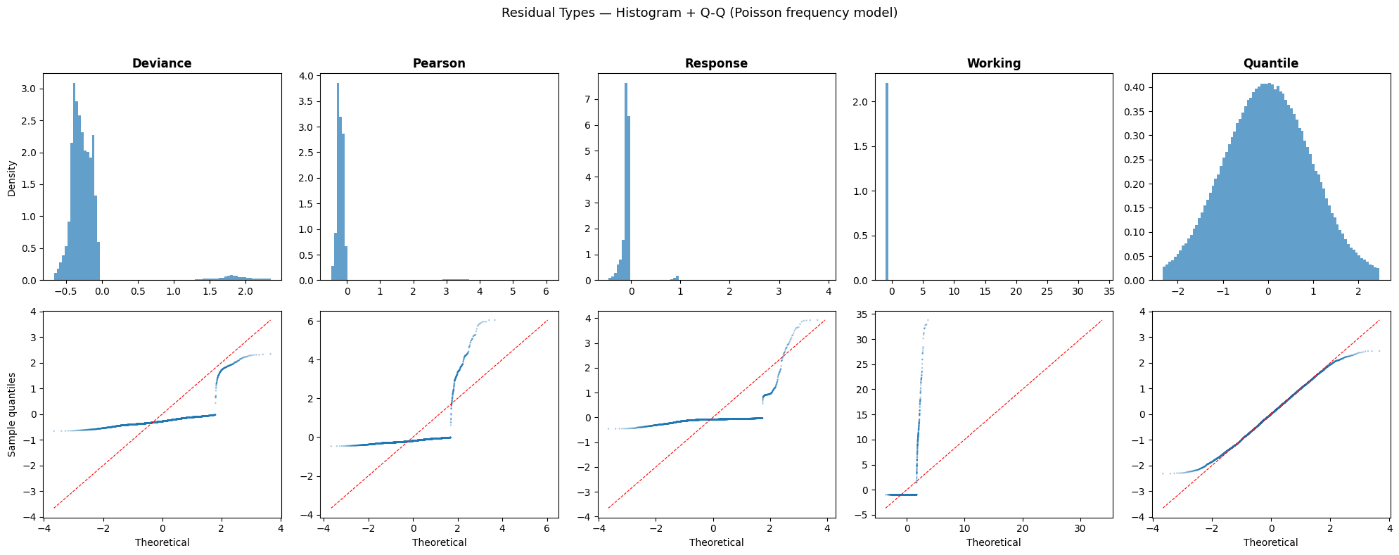
Compare all 5 residual types side by side: deviance, pearson, response, working, quantile. Shows distribution shape + Q-Q for each.

t0 = time.perf_counter()
m = model.metrics(X, y, exposure)
resid_types = ["deviance", "pearson", "response", "working", "quantile"]

fig, axes = plt.subplots(2, 5, figsize=(20, 8))

for i, rtype in enumerate(resid_types):
    r = m.residuals(rtype, seed=42)

    # Top row: histogram
    ax_h = axes[0, i]
    finite = r[np.isfinite(r)]
    lo, hi = np.percentile(finite, [1, 99])
    clipped = finite[(finite >= lo) & (finite <= hi)]
    ax_h.hist(clipped, bins=80, density=True, alpha=0.7, color="C0", edgecolor="none")
    ax_h.set_title(rtype.capitalize(), fontweight="bold")
    if i == 0:
        ax_h.set_ylabel("Density")

    # Bottom row: Q-Q
    ax_q = axes[1, i]
    n_qq = min(len(clipped), 5000)
    rng = np.random.default_rng(42)
    sample = rng.choice(clipped, n_qq, replace=False)
    sample.sort()
    theoretical = stats.norm.ppf((np.arange(1, n_qq + 1) - 0.375) / (n_qq + 0.25))
    ax_q.scatter(theoretical, sample, s=3, alpha=0.4, color="C0", edgecolors="none")
    lims = [min(theoretical.min(), sample.min()), max(theoretical.max(), sample.max())]
    ax_q.plot(lims, lims, "r--", linewidth=0.8)
    ax_q.set_xlabel("Theoretical")
    if i == 0:
        ax_q.set_ylabel("Sample quantiles")

fig.suptitle("Residual Types — Histogram + Q-Q (Poisson frequency model)", fontsize=13)
fig.tight_layout(rect=[0, 0, 1, 0.95])
plt.show()
print(f"[{time.perf_counter() - t0:.2f}s]")

[10.41s]

5b. Standardized & leverage metrics

print(
    f"Std deviance residuals — mean: {m.std_deviance_residuals.mean():.4f}, "
    f"std: {m.std_deviance_residuals.std():.4f}"
)
print(
    f"Std Pearson residuals  — mean: {m.std_pearson_residuals.mean():.4f}, "
    f"std: {m.std_pearson_residuals.std():.4f}"
)
print(f"Leverage — mean: {m.leverage.mean():.6f}, max: {m.leverage.max():.6f}")
print(
    f"Cook's D — mean: {m.cooks_distance.mean():.6f}, "
    f"max: {m.cooks_distance.max():.6f}, "
    f">0.5: {(m.cooks_distance > 0.5).sum()}, "
    f">1.0: {(m.cooks_distance > 1.0).sum()}"
)
print(f"Effective df: {m.effective_df:.1f}")
print(f"Phi (dispersion): {m.phi:.4f}")

Std deviance residuals — mean: -0.1757, std: 0.5302
Std Pearson residuals  — mean: 0.0482, std: 1.4413
Leverage — mean: 0.000093, max: 0.023952
Cook's D — mean: 0.000002, max: 0.001440, >0.5: 0, >1.0: 0
Effective df: 64.2
Phi (dispersion): 1.0000

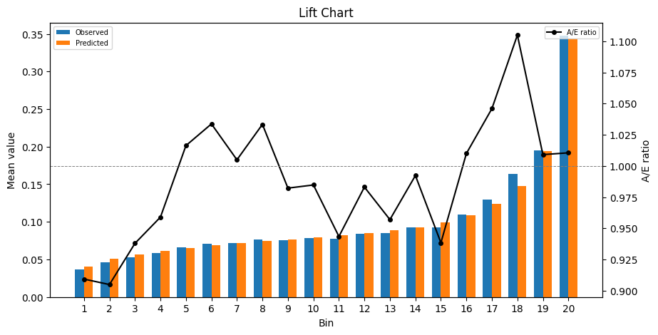
6. Lift chart

Observed vs predicted by equal-exposure quantile bins. A/E ratio on secondary axis.
Currently matplotlib only.

t0 = time.perf_counter()
result = lift_chart(
    y_obs=y,
    y_pred=mu,
    sample_weight=np.ones_like(y),
    exposure=exposure,
    n_bins=20,
)
plt.gcf().set_size_inches(10, 5)
plt.show()
print(result.bins.to_string(index=False))
print(f"[{time.perf_counter() - t0:.2f}s]")

 bin  exposure_share  observed  predicted  obs_pred_ratio
   1        0.049998  0.037153   0.040859        0.909300
   2        0.050002  0.046075   0.050917        0.904894
   3        0.049998  0.053274   0.056801        0.937915
   4        0.050001  0.058906   0.061426        0.958961
   5        0.050000  0.066325   0.065261        1.016309
   6        0.049999  0.070845   0.068535        1.033695
   7        0.050000  0.071792   0.071439        1.004938
   8        0.050001  0.076644   0.074171        1.033334
   9        0.049999  0.075475   0.076841        0.982222
  10        0.050001  0.078261   0.079473        0.984753
  11        0.049998  0.077542   0.082190        0.943449
  12        0.050001  0.083729   0.085173        0.983049
  13        0.050000  0.084846   0.088660        0.956977
  14        0.050001  0.092319   0.093034        0.992309
  15        0.050000  0.092934   0.099031        0.938429
  16        0.049999  0.109505   0.108420        1.010009
  17        0.050002  0.129355   0.123674        1.045937
  18        0.050000  0.163275   0.147768        1.104937
  19        0.050000  0.195462   0.193701        1.009094
  20        0.050000  0.347580   0.343962        1.010518
[0.43s]

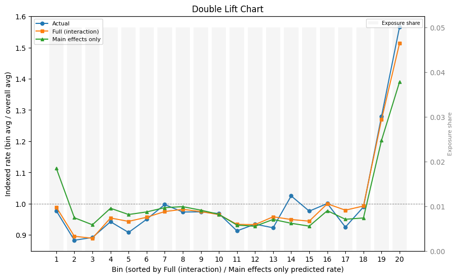
7. Double lift chart

Compare the full model (with interaction) against a main-effects-only model.

t0 = time.perf_counter()

# Fit a simpler main-effects-only model for comparison
model_simple = SuperGLM(
    family=Poisson(),
    selection_penalty=0,
    discrete=True,
    features={
        "DrivAge": Spline(n_knots=10, penalty="ssp"),
        "VehAge": Spline(n_knots=8, penalty="ssp"),
        "BonusMalus": Spline(n_knots=8, penalty="ssp"),
        "LogDensity": Spline(n_knots=7, penalty="ssp"),
        "Area": Categorical(base="first"),
        "VehPower": Spline(n_knots=7, penalty="ssp"),
    },
)
model_simple.fit_reml(X, y, sample_weight=exposure, max_reml_iter=6)
mu_simple = model_simple.predict(X)

print("=== Main-effects-only model ===")
model_simple.summary()

# CAS-style double lift chart
result = double_lift_chart(
    y_obs=y,
    y_pred_model=mu,
    y_pred_current=mu_simple,
    exposure=exposure,
    n_bins=20,
    labels=("Actual", "Full (interaction)", "Main effects only"),
)
plt.gcf().set_size_inches(10, 6)
plt.show()

# Audit table
print(
    result.bins[
        [
            "bin",
            "n_rows",
            "exposure_sum",
            "exposure_share",
            "actual_index",
            "model_index",
            "current_index",
            "sort_score_min",
            "sort_score_median",
            "sort_score_max",
        ]
    ].to_string(index=False)
)
print(f"[{time.perf_counter() - t0:.2f}s]")

=== Main-effects-only model ===
 bin  n_rows  exposure_sum  exposure_share  actual_index  model_index  current_index  sort_score_min  sort_score_median  sort_score_max
   1   36659      17926.58        0.050000      0.977376     0.989022       1.113485        0.639698           0.914333        0.927261
   2   35295      17926.75        0.050000      0.883069     0.895789       0.955182        0.927261           0.937906        0.946437
   3   34948      17926.11        0.049998      0.891976     0.889442       0.932621        0.946437           0.953365        0.961720
   4   34738      17927.30        0.050002      0.942392     0.954334       0.985522        0.961720           0.968265        0.974096
   5   31636      17926.49        0.049999      0.908043     0.943513       0.965432        0.974096           0.977355        0.979979
   6   31121      17926.78        0.050000      0.950185     0.956725       0.973753        0.979979           0.982481        0.984994
   7   31912      17926.78        0.050000      0.997334     0.974882       0.987488        0.984994           0.987307        0.989439
   8   32218      17926.47        0.049999      0.973499     0.982108       0.990621        0.989439           0.991485        0.993296
   9   32938      17926.77        0.050000      0.974037     0.974764       0.979394        0.993296           0.995281        0.997254
  10   33689      17926.70        0.050000      0.968494     0.965164       0.966113        0.997254           0.999028        1.000794
  11   33969      17927.09        0.050001      0.913005     0.933901       0.931643        1.000794           1.002472        1.004003
  12   34329      17926.66        0.050000      0.934660     0.933128       0.927937        1.004003           1.005565        1.007232
  13   34388      17926.12        0.049998      0.923039     0.958184       0.949656        1.007232           1.008919        1.010852
  14   33734      17927.14        0.050001      1.025048     0.949533       0.937391        1.010852           1.012993        1.015035
  15   33059      17926.69        0.050000      0.976260     0.944250       0.928229        1.015035           1.017195        1.019604
  16   32577      17926.61        0.050000      1.000671     0.999800       0.977747        1.019605           1.022346        1.026096
  17   32576      17926.65        0.050000      0.925231     0.979364       0.950220        1.026096           1.030834        1.035227
  18   32967      17926.29        0.049999      0.989595     0.992638       0.954413        1.035227           1.039652        1.045407
  19   36091      17927.29        0.050002      1.279635     1.269285       1.202872        1.045408           1.055400        1.065101
  20   39169      17926.96        0.050001      1.566430     1.514155       1.390270        1.065102           1.081179        1.272113
[4.56s]

8. Lorenz curve + Gini coefficient

Lorenz curve with model, perfect-foresight, and random ordering.
Gini ratio = model Gini / perfect Gini.

t0 = time.perf_counter()
result = lorenz_curve(
    y_obs=y,
    y_pred=mu,
    exposure=exposure,
)
plt.gcf().set_size_inches(7, 7)
plt.show()

print(f"Gini (model):   {result.gini_model:.4f}")
print(f"Gini (perfect): {result.gini_perfect:.4f}")
print(f"Gini ratio:     {result.gini_ratio:.4f}")
print(f"[{time.perf_counter() - t0:.2f}s]")

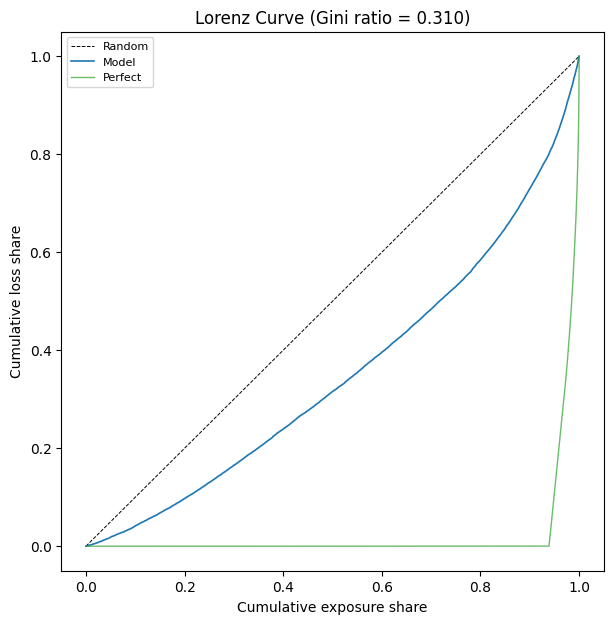
Gini (model):   0.2972
Gini (perfect): 0.9586
Gini ratio:     0.3101
[0.76s]

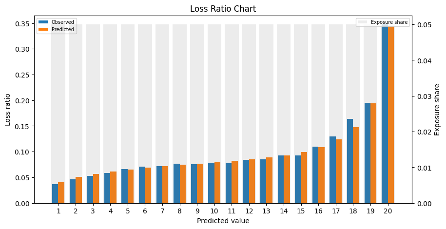
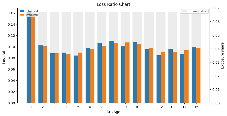
9. Loss ratio chart

Observed vs predicted loss ratios per quantile bin, with exposure share overlay.
Can bin by predicted value or by a specific feature.

t0 = time.perf_counter()
result = loss_ratio_chart(
    y_obs=y,
    y_pred=mu,
    exposure=exposure,
    n_bins=20,
)
plt.gcf().set_size_inches(10, 5)
plt.show()
print(f"[{time.perf_counter() - t0:.2f}s]")

[0.27s]

t0 = time.perf_counter()
result = loss_ratio_chart(
    y_obs=y,
    y_pred=mu,
    exposure=exposure,
    n_bins=15,
    feature_values=X["DrivAge"].to_numpy(),
    feature_name="DrivAge",
)
plt.gcf().set_size_inches(10, 5)
plt.show()
print(f"[{time.perf_counter() - t0:.2f}s]")

[0.21s]

10. Term importance

Weighted variance of each term’s contribution — how much each feature moves the linear predictor.

t0 = time.perf_counter()
importance = term_importance(model, X, sample_weight=exposure)
print(importance.to_string())
print(f"[{time.perf_counter() - t0:.2f}s]")

             term         feature subgroup_type  variance_eta    sd_eta        edf        lambda  group_norm
0         DrivAge         DrivAge          None      0.036953  0.192231   9.341341     12.179056    0.325179
1          VehAge          VehAge          None      0.088393  0.297310  10.829624      0.065387    3.889032
2      BonusMalus      BonusMalus          None      0.134949  0.367354   9.655321      0.485340    1.386007
3      LogDensity      LogDensity          None      0.003426  0.058528   1.222935  13357.538259    0.058742
4            Area            Area          None      0.000252  0.015866   5.000000           NaN    0.056427
5        VehPower        VehPower          None      0.007349  0.085725   8.456298      1.172102    0.802230
6  DrivAge:VehAge  DrivAge:VehAge          None      0.001734  0.041638  18.672645     34.276986    0.230864
[8.69s]

t0 = time.perf_counter()
feat_imp = importance.groupby("feature")["variance_eta"].sum()
feat_imp_pct = 100 * feat_imp / feat_imp.sum()
feat_imp_pct = feat_imp_pct.sort_values()

fig = go.Figure(
    go.Bar(
        x=feat_imp_pct.values,
        y=feat_imp_pct.index,
        orientation="h",
        marker_color="#1f77b4",
    )
)
fig.update_layout(
    title="Term Importance (% of weighted variance in linear predictor)",
    xaxis_title="Importance (%)",
    height=400,
    margin=dict(l=120),
)
fig.show()
print(f"[{time.perf_counter() - t0:.2f}s]")

[0.01s]

11. Cross-validation & holdout evaluation

CV for model selection and stability, holdout for final business-facing validation.

1. Split: 80% training, 20% untouched holdout

2. 5-fold CV on training for both models (same folds)

3. Compare fold-level and OOF metrics

4. Refit on all training data, final holdout double-lift chart

from sklearn.model_selection import KFold

from superglm.model_selection import cross_validate
from superglm.validation import lorenz_curve as _lorenz

t0 = time.perf_counter()

# ── Train/holdout split (80/20, shuffled, fixed seed) ─────────
rng_split = np.random.default_rng(42)
n_total = len(y)
idx_all = np.arange(n_total)
rng_split.shuffle(idx_all)
n_train = int(0.8 * n_total)
train_idx, holdout_idx = idx_all[:n_train], idx_all[n_train:]

X_train, X_holdout = (
    X.iloc[train_idx].reset_index(drop=True),
    X.iloc[holdout_idx].reset_index(drop=True),
)
y_train, y_holdout = y[train_idx], y[holdout_idx]
exp_train, exp_holdout = exposure[train_idx], exposure[holdout_idx]

print(f"Training: {len(y_train):,} rows, Holdout: {len(y_holdout):,} rows")
print(f"[{time.perf_counter() - t0:.2f}s]")

Training: 542,410 rows, Holdout: 135,603 rows
[0.04s]

t0 = time.perf_counter()

# ── Define models (unfitted) ──────────────────────────────────
model_full_cv = SuperGLM(
    family=Poisson(),
    selection_penalty=0,
    discrete=True,
    features={
        "DrivAge": Spline(n_knots=10, penalty="ssp"),
        "VehAge": Spline(n_knots=8, penalty="ssp"),
        "BonusMalus": Spline(n_knots=8, penalty="ssp"),
        "LogDensity": Spline(n_knots=7, penalty="ssp"),
        "Area": Categorical(base="first"),
        "VehPower": Spline(n_knots=7, penalty="ssp"),
    },
    interactions=[("DrivAge", "VehAge")],
)

model_simple_cv = SuperGLM(
    family=Poisson(),
    selection_penalty=0,
    discrete=True,
    features={
        "DrivAge": Spline(n_knots=10, penalty="ssp"),
        "VehAge": Spline(n_knots=8, penalty="ssp"),
        "BonusMalus": Spline(n_knots=8, penalty="ssp"),
        "LogDensity": Spline(n_knots=7, penalty="ssp"),
        "Area": Categorical(base="first"),
        "VehPower": Spline(n_knots=7, penalty="ssp"),
    },
)

# ── Same folds for both models ────────────────────────────────
splitter = KFold(n_splits=5, shuffle=True, random_state=42)
scoring = ("deviance", "nll", "gini")

# ── CV: full model ───────────────────────────────────────────
cv_full = cross_validate(
    model_full_cv,
    X_train,
    y_train,
    cv=splitter,
    sample_weight=exp_train,
    fit_mode="fit_reml",
    scoring=scoring,
    return_oof=True,
)
print(f"Full model CV: {time.perf_counter() - t0:.1f}s")

t1 = time.perf_counter()
# ── CV: simple model ─────────────────────────────────────────
cv_simple = cross_validate(
    model_simple_cv,
    X_train,
    y_train,
    cv=splitter,
    sample_weight=exp_train,
    fit_mode="fit_reml",
    scoring=scoring,
    return_oof=True,
)
print(f"Simple model CV: {time.perf_counter() - t1:.1f}s")
print(f"Total CV time: {time.perf_counter() - t0:.1f}s")

Full model CV: 42.4s
Simple model CV: 10.9s
Total CV time: 53.3s

# ── Fold-level results ────────────────────────────────────────
display_cols = [
    "fold",
    "n_train",
    "n_test",
    "fit_time_s",
    "converged",
    "n_iter",
    "effective_df",
    "deviance",
    "nll",
    "gini",
]

print("=== Full model (with interaction) — fold scores ===")
print(cv_full.fold_scores[display_cols].to_string(index=False))
print()
print("=== Simple model (main effects only) — fold scores ===")
print(cv_simple.fold_scores[display_cols].to_string(index=False))

=== Full model (with interaction) — fold scores ===
 fold  n_train  n_test  fit_time_s  converged  n_iter  effective_df  deviance      nll     gini
    0   433928  108482    2.862054       True       2     57.768299  0.588229 0.364239 0.289075
    1   433928  108482    2.803167       True       2     59.960673  0.608232 0.375039 0.282080
    2   433928  108482    2.899427       True       2     59.686495  0.591864 0.364801 0.299869
    3   433928  108482    2.888848       True       2     61.520812  0.584747 0.361082 0.287616
    4   433928  108482    3.444041       True       2     59.185172  0.578321 0.357496 0.308796

=== Simple model (main effects only) — fold scores ===
 fold  n_train  n_test  fit_time_s  converged  n_iter  effective_df  deviance      nll     gini
    0   433928  108482    1.119350       True       2     44.072253  0.588479 0.364364 0.289306
    1   433928  108482    1.058617       True       2     44.436972  0.608376 0.375111 0.282488
    2   433928  108482    1.081241       True       2     44.152330  0.592051 0.364895 0.300721
    3   433928  108482    0.962815       True       2     47.568499  0.585028 0.361222 0.287485
    4   433928  108482    1.140216       True       2     43.468669  0.578426 0.357548 0.309734

# ── Summary + paired comparison table ─────────────────────────
metrics = ["deviance", "nll", "gini"]
rows = []
for metric in metrics:
    f = cv_full.fold_scores[metric]
    s = cv_simple.fold_scores[metric]
    delta = f - s  # full minus simple

    rows.append(
        {
            "metric": metric,
            "better_when": "higher" if metric == "gini" else "lower",
            "full_mean": f"{f.mean():.4f}",
            "simple_mean": f"{s.mean():.4f}",
            "full_minus_simple_mean": f"{delta.mean():+.4f}",
            "full_median": f"{f.median():.4f}",
            "simple_median": f"{s.median():.4f}",
            "full_minus_simple_median": f"{delta.median():+.4f}",
            "delta_std": f"{delta.std():.4f}",
        }
    )

comparison = pd.DataFrame(rows)
print("=== Model comparison (full minus simple) ===")
print(comparison.to_string(index=False))
print()
print("Interpretation:")
print("  deviance/nll: lower is better, so negative full_minus_simple favors full")
print("  gini: higher is better, so positive full_minus_simple favors full")
print("  Very small deltas mean the global CV picture is basically a tie.")

=== Model comparison (full minus simple) ===
  metric better_when full_mean simple_mean full_minus_simple_mean full_median simple_median full_minus_simple_median delta_std
deviance       lower    0.5903      0.5905                -0.0002      0.5882        0.5885                  -0.0002    0.0001
     nll       lower    0.3645      0.3646                -0.0001      0.3642        0.3644                  -0.0001    0.0000
    gini      higher    0.2935      0.2939                -0.0005      0.2891        0.2893                  -0.0004    0.0004

Interpretation:
  deviance/nll: lower is better, so negative full_minus_simple favors full
  gini: higher is better, so positive full_minus_simple favors full
  Very small deltas mean the global CV picture is basically a tie.

# ── OOF overall metrics ───────────────────────────────────────
from superglm.distributions import Poisson as _Pois

oof_full = cv_full.oof_predictions
oof_simple = cv_simple.oof_predictions


def _oof_deviance(y, mu, w):
    fam = _Pois()
    return float(np.sum(w * fam.deviance_unit(y, mu)))


def _oof_gini(y, mu, w):
    result = _lorenz(y, mu, exposure=w)
    plt.close()  # don't display the lorenz figure
    return result.gini_ratio


print("=== OOF overall metrics (full training sample, every row scored out-of-fold) ===")
print(f"{'':20s} {'Full':>10s} {'Simple':>10s}")
print(
    f"{'OOF deviance':20s} {_oof_deviance(y_train, oof_full, exp_train):10.1f} {_oof_deviance(y_train, oof_simple, exp_train):10.1f}"
)
print(
    f"{'OOF Gini ratio':20s} {_oof_gini(y_train, oof_full, exp_train):10.4f} {_oof_gini(y_train, oof_simple, exp_train):10.4f}"
)

=== OOF overall metrics (full training sample, every row scored out-of-fold) ===
                           Full     Simple
OOF deviance           169213.9   169269.4
OOF Gini ratio           0.3058     0.3063

Holdout evaluation

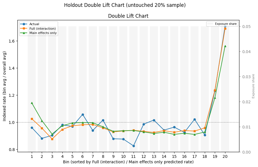
Refit both models on all training data, score the untouched holdout once, and build the final CAS-style double-lift chart.

t0 = time.perf_counter()

# ── Refit on all training data ────────────────────────────────
model_full_final = SuperGLM(
    family=Poisson(),
    selection_penalty=0,
    discrete=True,
    features={
        "DrivAge": Spline(n_knots=10, penalty="ssp"),
        "VehAge": Spline(n_knots=8, penalty="ssp"),
        "BonusMalus": Spline(n_knots=8, penalty="ssp"),
        "LogDensity": Spline(n_knots=7, penalty="ssp"),
        "Area": Categorical(base="first"),
        "VehPower": Spline(n_knots=7, penalty="ssp"),
    },
    interactions=[("DrivAge", "VehAge")],
)
model_full_final.fit_reml(X_train, y_train, sample_weight=exp_train, max_reml_iter=6)

model_simple_final = SuperGLM(
    family=Poisson(),
    selection_penalty=0,
    discrete=True,
    features={
        "DrivAge": Spline(n_knots=10, penalty="ssp"),
        "VehAge": Spline(n_knots=8, penalty="ssp"),
        "BonusMalus": Spline(n_knots=8, penalty="ssp"),
        "LogDensity": Spline(n_knots=7, penalty="ssp"),
        "Area": Categorical(base="first"),
        "VehPower": Spline(n_knots=7, penalty="ssp"),
    },
)
model_simple_final.fit_reml(X_train, y_train, sample_weight=exp_train, max_reml_iter=6)

# ── Score holdout ─────────────────────────────────────────────
mu_holdout_full = model_full_final.predict(X_holdout)
mu_holdout_simple = model_simple_final.predict(X_holdout)

print(f"Refit time: {time.perf_counter() - t0:.1f}s")
print(f"Holdout mean predicted (full):   {np.average(mu_holdout_full, weights=exp_holdout):.4f}")
print(f"Holdout mean predicted (simple): {np.average(mu_holdout_simple, weights=exp_holdout):.4f}")
print(f"Holdout mean observed:           {np.average(y_holdout, weights=exp_holdout):.4f}")

# ── Holdout Gini ──────────────────────────────────────────────
gini_full = _oof_gini(y_holdout, mu_holdout_full, exp_holdout)
gini_simple = _oof_gini(y_holdout, mu_holdout_simple, exp_holdout)
print(f"Holdout Gini (full):   {gini_full:.4f}")
print(f"Holdout Gini (simple): {gini_simple:.4f}")

# ── Final holdout double-lift chart ───────────────────────────
result_holdout = double_lift_chart(
    y_obs=y_holdout,
    y_pred_model=mu_holdout_full,
    y_pred_current=mu_holdout_simple,
    exposure=exp_holdout,
    n_bins=20,
    labels=("Actual", "Full (interaction)", "Main effects only"),
)
plt.gcf().set_size_inches(10, 6)
plt.suptitle("Holdout Double Lift Chart (untouched 20% sample)", fontsize=12)
plt.show()

print(
    result_holdout.bins[
        [
            "bin",
            "n_rows",
            "exposure_share",
            "actual_index",
            "model_index",
            "current_index",
            "sort_score_median",
        ]
    ].to_string(index=False)
)
print(f"[{time.perf_counter() - t0:.2f}s]")

Refit time: 6.4s
Holdout mean predicted (full):   0.1007
Holdout mean predicted (simple): 0.1007
Holdout mean observed:           0.1010
Holdout Gini (full):   0.3140
Holdout Gini (simple): 0.3133
 bin  n_rows  exposure_share  actual_index  model_index  current_index  sort_score_median
   1    7305        0.049998      0.961613     1.026365       1.143579           0.925420
   2    7219        0.049996      0.881735     0.957018       1.012312           0.945802
   3    6889        0.050005      0.903612     0.877108       0.913480           0.960414
   4    7040        0.050000      0.980848     0.947139       0.974576           0.972079
   5    6423        0.049999      0.969855     0.974719       0.995392           0.979449
   6    6352        0.049990      1.058200     0.981663       0.997947           0.983821
   7    6487        0.049999      0.939541     0.984772       0.996936           0.987951
   8    6693        0.050003      1.016598     0.958599       0.966717           0.991735
   9    6688        0.050008      0.878774     0.929195       0.934152           0.994804
  10    6772        0.050000      0.876151     0.936191       0.938136           0.998038
  11    6770        0.049990      0.826723     0.940993       0.939653           1.001521
  12    6724        0.050000      0.986367     0.933492       0.928984           1.004998
  13    6732        0.050009      1.016482     0.924998       0.917408           1.008374
  14    6576        0.049997      0.942328     0.938584       0.926978           1.012557
  15    6341        0.049999      0.964333     0.926624       0.910966           1.017320
  16    6295        0.050004      0.925678     0.939239       0.919338           1.021670
  17    6421        0.049993      1.022316     0.935214       0.910661           1.027082
  18    6162        0.050003      0.906398     0.959059       0.928368           1.032932
  19    7087        0.049996      1.231677     1.236956       1.181132           1.047372
  20    8627        0.050009      1.710655     1.691977       1.563221           1.072164
[6.63s]

More proof

Add two stronger pieces of evidence:

1. repeated CV on the same training sample with different shuffle seeds

2. a holdout tail-error summary showing how much closer each model is to Actual in the top lift bins

t0 = time.perf_counter()

# ── Repeated CV stability check (same 80% training sample) ────
# Keep repeats modest for demo speed; increase if you want tighter evidence.
repeat_seeds = [7, 42, 99]
repeat_rows = []

for seed in repeat_seeds:
    splitter = KFold(n_splits=5, shuffle=True, random_state=seed)

    r_full = cross_validate(
        model_full_cv,
        X_train,
        y_train,
        cv=splitter,
        sample_weight=exp_train,
        fit_mode="fit_reml",
        scoring=scoring,
        return_oof=False,
    )
    r_simple = cross_validate(
        model_simple_cv,
        X_train,
        y_train,
        cv=splitter,
        sample_weight=exp_train,
        fit_mode="fit_reml",
        scoring=scoring,
        return_oof=False,
    )

    row = {
        "seed": seed,
        "full_edf": float(r_full.fold_scores["effective_df"].mean()),
        "simple_edf": float(r_simple.fold_scores["effective_df"].mean()),
        "delta_edf": float(
            r_full.fold_scores["effective_df"].mean() - r_simple.fold_scores["effective_df"].mean()
        ),
    }
    for metric in metrics:
        full_mean = float(r_full.fold_scores[metric].mean())
        simple_mean = float(r_simple.fold_scores[metric].mean())
        row[f"full_{metric}"] = full_mean
        row[f"simple_{metric}"] = simple_mean
        row[f"delta_{metric}"] = full_mean - simple_mean
    repeat_rows.append(row)

repeat_df = pd.DataFrame(repeat_rows)
print("=== Repeated 5-fold CV (same training sample, different shuffle seeds) ===")
print(repeat_df.to_string(index=False, float_format=lambda x: f"{x:.4f}"))
print()

summary_rows = []
for metric in metrics:
    delta = repeat_df[f"delta_{metric}"]
    summary_rows.append(
        {
            "metric": metric,
            "better_when": "higher" if metric == "gini" else "lower",
            "delta_mean": float(delta.mean()),
            "delta_median": float(delta.median()),
            "delta_std": float(delta.std(ddof=0)),
        }
    )

repeat_summary = pd.DataFrame(summary_rows)
print("=== Stability summary across repeated CV runs ===")
print(
    repeat_summary.to_string(
        index=False, float_format=lambda x: f"{x:+.4f}" if abs(x) < 10 else f"{x:.4f}"
    )
)
print()
print("Interpretation:")
print("  deviance/nll: lower is better, so negative delta favors full")
print("  gini: higher is better, so negative delta favors simple")
print(
    "  Here the global CV differences are tiny: full is slightly better on deviance/nll, simple is slightly better on gini."
)
print(f"  mean EDF delta (full - simple): {repeat_df['delta_edf'].mean():+.2f}")
print(f"[{time.perf_counter() - t0:.1f}s]")

=== Repeated 5-fold CV (same training sample, different shuffle seeds) ===
 seed  full_edf  simple_edf  delta_edf  full_deviance  simple_deviance  delta_deviance  full_nll  simple_nll  delta_nll  full_gini  simple_gini  delta_gini
    7   59.6849     44.3185    15.3664         0.5903           0.5904         -0.0002    0.3645      0.3646    -0.0001     0.2935       0.2941     -0.0007
   42   59.6243     44.7397    14.8845         0.5903           0.5905         -0.0002    0.3645      0.3646    -0.0001     0.2935       0.2939     -0.0005
   99   59.6952     44.5058    15.1894         0.5903           0.5905         -0.0002    0.3645      0.3646    -0.0001     0.2934       0.2940     -0.0006

=== Stability summary across repeated CV runs ===
  metric better_when  delta_mean  delta_median  delta_std
deviance       lower     -0.0002       -0.0002    +0.0000
     nll       lower     -0.0001       -0.0001    +0.0000
    gini      higher     -0.0006       -0.0006    +0.0001

Interpretation:
  deviance/nll: lower is better, so negative delta favors full
  gini: higher is better, so negative delta favors simple
  Here the global CV differences are tiny: full is slightly better on deviance/nll, simple is slightly better on gini.
  mean EDF delta (full - simple): +15.15
[134.2s]

# ── Holdout tail-error summary ────────────────────────────────
bins = result_holdout.bins.copy()
bins["full_abs_err"] = (bins["actual_index"] - bins["model_index"]).abs()
bins["simple_abs_err"] = (bins["actual_index"] - bins["current_index"]).abs()


def _weighted_err(df, col):
    return float(np.average(df[col], weights=df["exposure_share"]))


tail_masks = {
    "all bins": bins["bin"] >= bins["bin"].min(),
    "top 3 bins": bins["bin"] >= bins["bin"].max() - 2,
    "top 2 bins": bins["bin"] >= bins["bin"].max() - 1,
    "top 1 bin": bins["bin"] == bins["bin"].max(),
}

rows = []
for label, mask in tail_masks.items():
    df = bins.loc[mask]
    full_err = _weighted_err(df, "full_abs_err")
    simple_err = _weighted_err(df, "simple_abs_err")
    improvement = simple_err - full_err
    improvement_pct = improvement / simple_err if simple_err > 0 else np.nan
    rows.append(
        {
            "segment": label,
            "full_abs_error": full_err,
            "simple_abs_error": simple_err,
            "error_reduction": improvement,
            "error_reduction_pct": improvement_pct,
        }
    )

tail_summary = pd.DataFrame(rows)
print("=== Holdout indexed-rate error summary ===")
print(tail_summary.to_string(index=False, float_format=lambda x: f"{x:.4f}"))
print()
print("=== Top holdout bins ===")
print(
    bins.loc[
        bins["bin"] >= bins["bin"].max() - 1,
        [
            "bin",
            "exposure_share",
            "actual_index",
            "model_index",
            "current_index",
            "sort_score_median",
        ],
    ].to_string(index=False)
)

=== Holdout indexed-rate error summary ===
   segment  full_abs_error  simple_abs_error  error_reduction  error_reduction_pct
  all bins          0.0486            0.0658           0.0171               0.2604
top 3 bins          0.0255            0.0733           0.0478               0.6517
top 2 bins          0.0120            0.0990           0.0870               0.8790
 top 1 bin          0.0187            0.1474           0.1288               0.8733

=== Top holdout bins ===
 bin  exposure_share  actual_index  model_index  current_index  sort_score_median
  19        0.049996      1.231677     1.236956       1.181132           1.047372
  20        0.050009      1.710655     1.691977       1.563221           1.072164

11. Summary

Plot	Backend	Status
Main effects explorer	Plotly	Full support
Main effects grid	Matplotlib	Full support
Interaction surface	Plotly	Full support
Interaction contour	Plotly	Full support
Interaction contour + HDR	Plotly	Full support
4-panel diagnostics	Matplotlib	Full support
Residual types (5)	Matplotlib	Full support
Lift chart	Matplotlib	No Plotly
Double lift chart	Matplotlib	No Plotly
Lorenz curve	Matplotlib	No Plotly
Loss ratio chart	Matplotlib	No Plotly
Term importance	Plotly (manual)	No built-in plot
Residual diagnostics	Matplotlib	No Plotly