Check the fit

The residual checks start from residuals(): the probability-integral transform of each row under its fitted law, or its normal inverse, which a correct family makes uniform or standard normal; residual_set() is the full payload the residual comes from. check() bins those residuals along a covariate and reports mean, standard deviation and skewness per bin with bootstrap bands, so it says where the fit is wrong and in which moment; check_2d() reports the mean on a grid of two covariates. actual_expected() reports realised against predicted totals per bin as a ratio of weighted sums, and calibration() answers the coverage, tail, quantile and reliability questions in one payload. scores() gives proper scores per row, the log score and the CRPS, and compare() the paired score difference against another fitted candidate. The how-to on checking a distributional fit reads each of these in turn.

residuals	Return one residual per row: "quantile" or the raw "pit" value.
residual_set	Return the full residual payload of y under the fitted parameters.
check	Return the mean, standard deviation and skewness of the residuals per bin.
check_2d	Return the mean residual on a two-dimensional grid of two covariates.
actual_expected	Return the realised against the predicted total per bin of a covariate.
calibration	Return interval coverage, tail totals, quantile calibration and reliability.
scores	Return one column of proper scores per requested rule, one row per row.
compare	Return the paired score difference against another fitted candidate.

Example

The same simulated severity book as the inference page: 3,000 claim amounts whose log-normal location peaks near age 30 and shifts by region, and whose scale widens with age.

import numpy as np
import pandas as pd

from superglm import LogNormalLS, SuperLSS, cat, s

rng = np.random.default_rng(1)
n = 3000
book = pd.DataFrame(
    {
        "age": rng.uniform(18, 80, n),
        "region": rng.choice(["North", "South", "East", "West"], n),
    }
)
age = book["age"].to_numpy()
by_region = book["region"].map(
    {"North": 0.0, "South": 0.25, "East": -0.15, "West": 0.1}
).to_numpy()
location = 7.0 + 0.9 * np.exp(-(((age - 30) / 14) ** 2)) + by_region
scale = 0.35 + 0.006 * (age - 18)
amount = np.exp(rng.normal(location, scale))

family = LogNormalLS(parametrisation="location")
model = SuperLSS(
    family,
    family.location(s("age", kind="cr", k=8), cat("region")),
    family.scale(s("age", kind="cr", k=6)),
).fit_reml(book, amount, outer="efs+newton")
model.smoothing_certified_

True

check bins the normalised residuals along a covariate and reports their mean, standard deviation and skewness per bin with bootstrap bands. A fit that has the location right puts the means on zero; one that has the spread right puts the standard deviations on one.

import matplotlib.pyplot as plt

checked = model.check(book, amount, "age", n_bins=10)

fig, axes = plt.subplots(2, 1, figsize=(6.4, 4.6), sharex=True)
for ax, value, lower, upper, target, label in (
    (
        axes[0],
        checked.mean,
        checked.mean_lower,
        checked.mean_upper,
        0.0,
        "residual mean",
    ),
    (axes[1], checked.sd, checked.sd_lower, checked.sd_upper, 1.0, "residual sd"),
):
    ax.fill_between(checked.centers, lower, upper, alpha=0.3)
    ax.plot(checked.centers, value, marker="o", markersize=3)
    ax.axhline(target, color="black", linewidth=0.8, linestyle="--")
    ax.set_ylabel(label)
axes[1].set_xlabel("age")
fig.tight_layout()

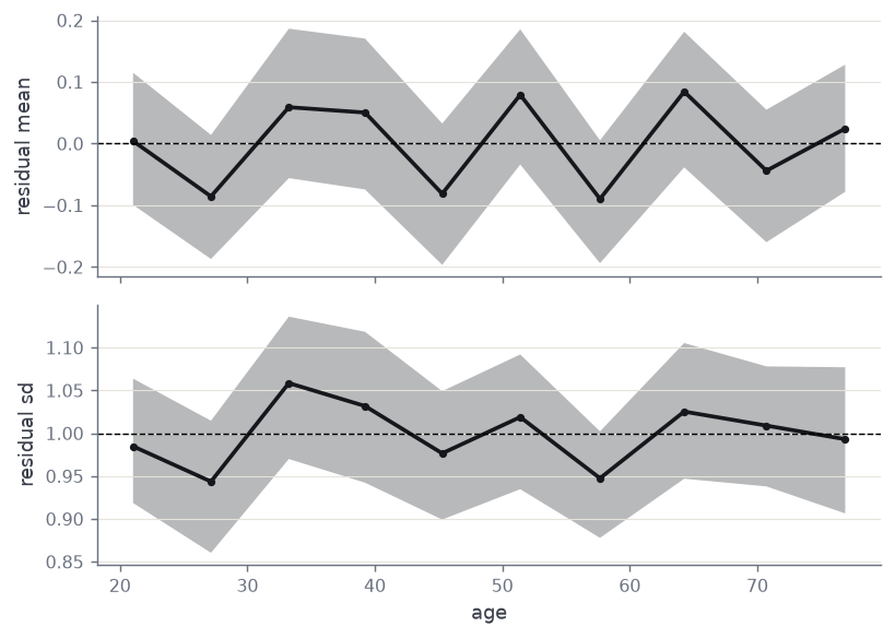
Both moments are where they should be across the whole age range: the binned means stay within 0.09 of zero and the standard deviations between 0.94 and 1.06, and every bin’s band covers its target. Had the scale been held constant the lower panel would tilt — small residual spread at young ages, large at old — which is exactly the failure the second panel exists to catch.

actual_expected leaves residual space and reports money: realised against predicted totals per level, as a ratio of weighted sums.

ae = model.actual_expected(book, amount, "region")
pd.DataFrame(
    {
        "level": ae.levels,
        "rows": ae.n,
        "actual": ae.actual,
        "expected": ae.expected,
        "ratio": ae.ratio,
        "ratio_se": ae.ratio_se,
    }
).round(3)

	level	rows	actual	expected	ratio	ratio_se
0	East	758	1203891.603	1198546.110	1.004	0.02
1	North	735	1338002.607	1338146.535	1.000	0.02
2	South	734	1735412.409	1713691.709	1.013	0.02
3	West	773	1549901.112	1566643.390	0.989	0.02

All four regions land within 1.3% of parity and every ratio is inside one standard error of one, so there is no region the fit is systematically underpricing.

scores gives proper scores per row; the mean log score is the average negative log-likelihood on these rows and the CRPS is in the units of the claim itself. Both are only meaningful against another candidate.

model.scores(book, amount).mean().round(3)

log       8.132
crps    540.606
dtype: float64

compare refits the same location predictor with one standard deviation for every row, then pairs the two fits row by row.

flat_scale = SuperLSS(
    family,
    family.location(s("age", kind="cr", k=8), cat("region")),
    family.scale(),
).fit_reml(book, amount, outer="efs+newton")

pd.Series(model.compare(flat_scale, book, amount, which="log").overall).round(4)

mean_diff      -0.0288
se              0.0043
t              -6.6775
n            3000.0000
dtype: float64

The mean log-score difference is -0.029 in favour of the varying-scale model, with a t statistic of -6.7 on 3,000 rows: the age effect on the spread is not a rounding artefact, and the check above is what it looks like when it is modelled.