Price and portfolio views

risk_curves() sweeps one covariate and returns predicted response quantiles with posterior bands drawn from one shared draw set, so the curves are coherent with one another; density_fan() is the same sweep but returns the whole conditional density at each point, the picture that shows a shape change; it supports continuous families only, and families with atoms refuse. parameter_spread() shows how far the fitted parameters spread across rows and, among identically priced rows, how far the tail probability does. portfolio() simulates the total over a book of rows, optionally by segment, carrying the dependence the shared coefficient draws induce.

risk_curves	Return predicted response quantiles along one covariate, with bands.
density_fan	Return the conditional response density along one covariate.
parameter_spread	Return how far the fitted parameters spread, and how far identical prices do.
portfolio	Return the simulated total over a book of rows, optionally by segment.

Example

The same simulated severity book as the inference page: 3,000 claim amounts whose log-normal location peaks near age 30 and shifts by region, and whose scale widens with age.

import numpy as np
import pandas as pd

from superglm import LogNormalLS, SuperLSS, cat, s

rng = np.random.default_rng(1)
n = 3000
book = pd.DataFrame(
    {
        "age": rng.uniform(18, 80, n),
        "region": rng.choice(["North", "South", "East", "West"], n),
    }
)
age = book["age"].to_numpy()
by_region = book["region"].map(
    {"North": 0.0, "South": 0.25, "East": -0.15, "West": 0.1}
).to_numpy()
location = 7.0 + 0.9 * np.exp(-(((age - 30) / 14) ** 2)) + by_region
scale = 0.35 + 0.006 * (age - 18)
amount = np.exp(rng.normal(location, scale))

family = LogNormalLS(parametrisation="location")
model = SuperLSS(
    family,
    family.location(s("age", kind="cr", k=8), cat("region")),
    family.scale(s("age", kind="cr", k=6)),
).fit_reml(book, amount, outer="efs+newton")
model.smoothing_certified_

True

A reference policy fixes every column but the one being swept. risk_curves then prices that policy across the age range and reports the median, the 90th and the 99th percentile of the claim it would bring, each with its posterior band.

import matplotlib.pyplot as plt

reference = pd.Series({"age": 45.0, "region": "North"})
curves = model.risk_curves(reference, "age")

fig, ax = plt.subplots(figsize=(6.4, 3.6))
for i, level in enumerate(curves.quantiles):
    line, = ax.plot(curves.x, curves.values[i], label=f"q{level:g}")
    ax.fill_between(
        curves.x, curves.lower[i], curves.upper[i], alpha=0.25, color=line.get_color()
    )
ax.set_xlabel("age")
ax.set_ylabel("claim amount")
ax.legend(loc="upper right", frameon=False)
fig.tight_layout()

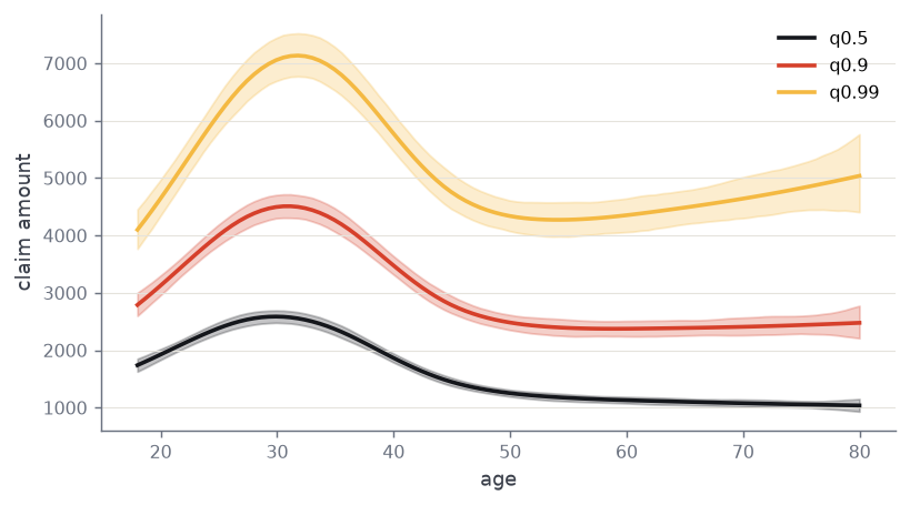
All three curves peak near age 30 and then separate. Between age 30 and age 75 the median falls to 41% of its age-30 value; the 99th percentile keeps 68% of its and turns back up past age 55. The location is shrinking and the scale is widening at the same time, so the older policy is cheaper on average and relatively more exposed in the tail. A mean-only model prices the first move and misses the second.

density_fan is the same sweep as the whole conditional density rather than three of its quantiles, with those quantiles drawn over it.

fan = model.density_fan(reference, "age")

fig, ax = plt.subplots(figsize=(6.4, 3.6))
mesh = ax.pcolormesh(fan.x, fan.y_grid, fan.density.T, cmap="Blues", shading="auto")
for i, level in enumerate(fan.quantile_levels):
    ax.plot(fan.x, fan.quantiles[i], linewidth=1.2, label=f"q{level:g}")
ax.set_ylim(0, 1.15 * float(np.max(fan.quantiles)))
ax.legend(loc="upper right", frameon=False)
ax.set_xlabel("age")
ax.set_ylabel("claim amount")
fig.colorbar(mesh, ax=ax, label="density")
fig.tight_layout()

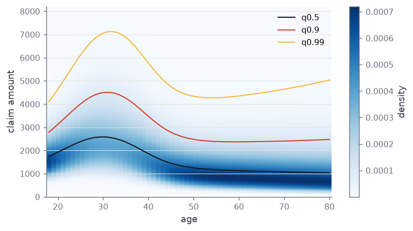
As age rises the mass sinks towards small claims and packs more tightly there, while the q0.99 line stops falling and lifts again: the law is not sliding down, it is growing more right-skewed. That is a shape change, and it is what the quantile curves above can only imply.

parameter_spread bins the book by predicted mean and asks how far the tail probability moves inside a bin, reporting its 5th and 95th percentiles per bin and their ratio.

spread = model.parameter_spread(book, threshold=5000.0)
priced = spread.identically_priced
widest = priced.loc[priced["ratio"].idxmax()]
pd.Series(
    {
        "bins": float(len(priced)),
        "median ratio across bins": priced["ratio"].median(),
        "widest ratio": widest["ratio"],
        "lowest mean in that bin": widest["mean_lo"],
        "highest mean in that bin": widest["mean_hi"],
        "5th percentile of P(Y > 5000)": widest["p_lo"],
        "95th percentile of P(Y > 5000)": widest["p_hi"],
    }
).round(5)

bins                                20.00000
median ratio across bins             2.78864
widest ratio                        33.71049
lowest mean in that bin           1605.27393
highest mean in that bin          1680.26551
5th percentile of P(Y > 5000)        0.00075
95th percentile of P(Y > 5000)       0.02524
dtype: float64

In the typical bin the chance of a claim above 5,000 varies by a factor of 2.8 between the 5th and the 95th percentile row; in the widest bin it varies by a factor of 34, from 0.00075 to 0.0252 at those two percentiles, while a mean-only model prices every row in that bin between 1,605 and 1,680. Those rows are priced as one risk and are not one risk.

portfolio simulates every row on its own predictive law and sums the draws, so the quantiles are of the book total.

total = model.portfolio(book, quantiles=(0.05, 0.5, 0.95))
pd.Series(
    {
        "observed": amount.sum(),
        "mean": total.total_mean,
        "sd": total.total_sd,
        "5%": total.total_quantiles[0.05],
        "50%": total.total_quantiles[0.5],
        "95%": total.total_quantiles[0.95],
    }
).round(0)

observed    5827208.0
mean        5823306.0
sd            82959.0
5%          5686034.0
50%         5821084.0
95%         5952288.0
dtype: float64

The expected total is 5.82 million against an observed 5.83 million, and the 5% to 95% interval spans 4.6% of the mean: the aggregate is far tighter than any single policy because the row draws average out, while the coefficient draws they share keep it from being tighter still.