Inference

summary() gives one row per intercept and per term of every parameter: effective degrees of freedom, smoothing parameter, the Wood (2013) statistic with its p-value and, for single-coefficient terms, the estimate and standard error. term_inference() sweeps one term of one parameter over its training range with pointwise and simultaneous bands, and term_test() is the test that the term is flat; all three read the training frame, so a model restored from bytes needs X_train=. The fitted attributes are the fit’s own state: coef_ and coef_by_predictor_, covariance_, smoothing_parameters_, result_, and the family_, predictors_ and parameter_names_ the fit resolved.

summary	Return one row per intercept and per term of every parameter.
term_inference	Return one term of one parameter on that parameter's link scale.
term_test	Return the Wood (2013) test that one term of one parameter is flat.
parameter_names_	Return fitted parameter names in the order used by predictions.
family_	Return an independent copy of the fitted family's configuration.
predictors_
coef_
coef_by_predictor_
covariance_
result_
smoothing_parameters_

Example

A simulated severity book of 3,000 claims. The location of the log-normal law rises to a peak near age 30 and shifts by region; its scale widens steadily with age. Both parameters carry real structure, so both predictors have something to find.

import numpy as np
import pandas as pd

from superglm import LogNormalLS, SuperLSS, cat, s

rng = np.random.default_rng(1)
n = 3000
book = pd.DataFrame(
    {
        "age": rng.uniform(18, 80, n),
        "region": rng.choice(["North", "South", "East", "West"], n),
    }
)
age = book["age"].to_numpy()
by_region = book["region"].map(
    {"North": 0.0, "South": 0.25, "East": -0.15, "West": 0.1}
).to_numpy()
location = 7.0 + 0.9 * np.exp(-(((age - 30) / 14) ** 2)) + by_region
scale = 0.35 + 0.006 * (age - 18)
amount = np.exp(rng.normal(location, scale))

family = LogNormalLS(parametrisation="location")
model = SuperLSS(
    family,
    family.location(s("age", kind="cr", k=8), cat("region")),
    family.scale(s("age", kind="cr", k=6)),
).fit_reml(book, amount, outer="efs+newton")
model.smoothing_certified_

True

The fit certified its smoothing parameters, so the summary below reads as a converged fit rather than a stopping point.

model.summary().round(3)

	parameter	term	edf	lambda	statistic	rank	p_value	estimate	se	note
0	location	(intercept)	1.000	NaN	163230.004	1.000	0.0	7.433	0.018
1	location	age	6.321	6641.042	1321.379	6.833	0.0	NaN	NaN
2	location	region	3.000	NaN	251.809	3.000	0.0	NaN	NaN
3	scale	(intercept)	1.000	NaN	2660.182	1.000	0.0	-0.679	0.013
4	scale	age	2.080	1040376.803	177.205	2.569	0.0	NaN	NaN

One row per intercept and per term of each parameter. The age smooth in location spends 6.3 effective degrees of freedom of the eight basis functions it was given; the age smooth in scale spends 2.1 of six, so the spread moves with age far more gently than the location does. Every term’s Wood statistic is large enough that its p-value rounds to zero at three decimal places.

term_inference returns one term of one parameter swept over its training range: the centred effect on the link scale, identity here, so log-amount units, with pointwise bounds and the simultaneous ones.

age_effect = model.term_inference("location", "age")
band = pd.DataFrame(
    {
        "age": age_effect.x,
        "effect": age_effect.effect,
        "lower": age_effect.lower,
        "upper": age_effect.upper,
        "lower_simultaneous": age_effect.lower_simultaneous,
        "upper_simultaneous": age_effect.upper_simultaneous,
    }
)
print(f"edf {age_effect.edf:.2f}, critical value {age_effect.critical_value:.2f}")
band.head().round(3)

edf 6.32, critical value 2.97

	age	effect	lower	upper	lower_simultaneous	upper_simultaneous
0	18.006	0.143	0.072	0.214	0.035	0.251
1	18.317	0.159	0.092	0.226	0.057	0.261
2	18.629	0.175	0.112	0.238	0.079	0.271
3	18.940	0.191	0.132	0.251	0.101	0.281
4	19.252	0.207	0.151	0.263	0.122	0.292

The simultaneous bounds use a critical value of 2.97 rather than the pointwise 1.96, which is why they sit further out at every age.

The same frame, drawn with both bands.

import matplotlib.pyplot as plt

fig, ax = plt.subplots(figsize=(6.4, 3.6))
ax.fill_between(
    band["age"],
    band["lower_simultaneous"],
    band["upper_simultaneous"],
    alpha=0.25,
    label="simultaneous",
)
ax.fill_between(
    band["age"], band["lower"], band["upper"], alpha=0.45, label="pointwise"
)
ax.plot(band["age"], band["effect"], color="black", linewidth=1.5, label="effect")
ax.set_xlabel("age")
ax.set_ylabel("location effect (log amount)")
ax.legend(loc="upper right", frameon=False)
fig.tight_layout()

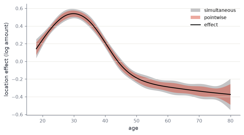
The curve peaks near age 30 and falls away on both sides, which is the shape the data were built with. The pointwise band answers “is the effect at this age different from the average?”; the simultaneous band, about 1.5 times as wide here, answers the question a pricing review actually asks — “could this whole curve have been flat?” — and a flat line does not fit inside it.

term_test asks the same question of the scale predictor, as a test rather than a picture.

test = model.term_test("scale", "age")
pd.Series(
    {
        "statistic": f"{test.statistic:.2f}",
        "rank": f"{test.rank:.2f}",
        "edf": f"{test.edf:.2f}",
        "p_value": f"{test.p_value:.1e}",
    }
)

statistic     177.20
rank            2.57
edf             2.08
p_value      1.2e-38
dtype: str

The statistic is 177 on 2.6 ranks and the p-value is far below any usual threshold, so the width of the claim distribution genuinely varies with age: a location-only model would misstate the tail at both ends of the age range.