
Inference#
Start with summary(), the statsmodels-style
coefficient table. term_inference() is the object
behind every curve and band, the per-term curve, uncertainty and metadata in
one place; simultaneous_bands() returns
simultaneous confidence bands for a spline feature, which hold jointly across
the curve. metrics() computes the fit statistics
and drop1() the drop-one deviance per feature;
term_importance() scores each term by the weighted
variance of its contribution to the linear predictor, and
term_drop_diagnostics() by what dropping it costs
in AIC, BIC or holdout loss. random_effects() and
factor_smooth() report variance components, level
diagnostics and smooth curves for random-effect and factor-smooth terms, while
knot_summary(),
design_summary() and the
result property expose what was actually built
and fitted.
Rich model summary with coefficient table (statsmodels-style). |
|
Per-term inference: curve, uncertainty, and metadata in one object. |
|
Simultaneous confidence bands for a spline feature. |
|
Return variance-component and per-level credibility diagnostics. |
|
Return basis-aware penalties, level diagnostics, and smooth curves. |
|
Compute comprehensive diagnostics for the fitted model. |
|
Drop-one deviance analysis for each feature. |
|
Weighted variance of each term's contribution to eta. |
|
Drop-term diagnostics: AIC/BIC deltas or holdout loss deltas. |
|
Return fitted knot metadata for all spline features. |
|
Describe fitted design storage and static route eligibility. |
|
The fitted public PIRLS result (canonical coefficients and fit stats). |
Example#
A simulated motor book: 4,000 policies, a non-linear age effect, four regions with different base rates, a mild vehicle-power slope, and Poisson claim counts whose rate is multiplied by exposure. The exposure enters as a log offset, so the model estimates a claim rate per unit of exposure.
import numpy as np
import pandas as pd

from superglm import Categorical, Numeric, Spline, SuperGLM

rng = np.random.default_rng(0)
n = 4000
region = rng.choice(["North", "South", "East", "West"], n, p=[0.35, 0.3, 0.2, 0.15])
age = rng.uniform(18, 80, n)
veh_power = rng.uniform(4, 12, n)
exposure = rng.uniform(0.1, 1.0, n)
region_effect = pd.Series(region).map(
    {"North": 0.0, "South": 0.25, "East": -0.2, "West": 0.4}
).to_numpy()
log_rate = (
    -1.2
    + 1.1 * np.exp(-((age - 24) ** 2) / 90.0)
    + 0.004 * (age - 50) ** 2 / 10.0
    + region_effect
    + 0.09 * (veh_power - 8)
)
claims = rng.poisson(np.exp(log_rate) * exposure)
X = pd.DataFrame({"age": age, "region": region, "veh_power": veh_power})
offset = np.log(exposure)

model = SuperGLM(
    family="poisson",
    features={
        "age": Spline(kind="cr", k=10),
        "region": Categorical(),
        "veh_power": Numeric(),
    },
).fit_reml(X, claims, offset=offset)
model.reml_diagnostics()["converged"]
True
summary is the whole fit in one table: the header block carries the family,
the effective degrees of freedom and the fit statistics, then each feature gets
its own section. A spline is reported as one block — its basis size, its
effective degrees of freedom, the smoothing parameter REML chose and a Wood
(2013) test — rather than as nine uninterpretable coefficients. The
categorical levels are shown against the reference level.
print(model.summary())
╔═════════════════════════════════ SuperGLM Results ═════════════════════════════════╗
║ Family:                          Poisson  No. Observations:                   4000 ║
║ Link:                                Log  Df (effective):     9.577 (4.577 smooth) ║
║ Method:                             REML  Penalty:                            None ║
║ Scale (phi):                       1.000  Pearson chi2:                     3991.9 ║
║ Log-Likelihood:                  -2563.7  AIC:                              5146.6 ║
║ AICc:                             5146.7  BIC:                              5206.9 ║
║ EBIC:                             5206.9  Converged:                 True (5 iter) ║
║ Deviance:                         2983.8                                           ║
╠════════════════════════════════════════════════════════════════════════════════════╣
║ Term                coef    std err        z    P>|z|    [0.025    0.975] Sig LC   ║
╟────────────────────────────────────────────────────────────────────────────────────╢
║ Intercept        -1.5888     0.1180  -13.468    0.000    -1.820    -1.358 *** ---  ║
║                                                                                    ║
╠══════════════════════════════════════╡ age ╞═══════════════════════════════════════╣
║                                                                                    ║
║ age            [spline, 9 params, chi2(5.6)=337.0, p=<0.001]              ***      ║
║                  rank=9, edf=4.6, lam=8.3e+03, curve SE: 0.05-0.13                 ║
║                                                                                    ║
╠═════════════════════════════════════╡ region ╞═════════════════════════════════════╣
║                                                                                    ║
║ region[East]     -0.2175     0.0909   -2.392    0.017    -0.396    -0.039 *   ---  ║
║ region[North]     0.0000        ref      ---      ---       ---       --- --- ---  ║
║ region[South]     0.3612     0.0687    5.254 1.49e-07     0.226     0.496 *** ---  ║
║ region[West]      0.4007     0.0830    4.826 1.39e-06     0.238     0.563 *** ---  ║
║                                                                                    ║
╠═══════════════════════════════════╡ veh_power ╞════════════════════════════════════╣
║                                                                                    ║
║ veh_power         0.0911     0.0123    7.404 1.33e-13     0.067     0.115 *** ---  ║
╚════════════════════════════════════════════════════════════════════════════════════╝
Signif. codes:  0 '***' 0.001 '**' 0.01 '*' 0.05 '.' 0.1 ' ' 1
Note: smooth p-values use Wood (2013) Bayesian test.
Parametric p-values are Wald approximations.
For borderline significance, use a likelihood ratio test.
term_inference is the object behind every curve and band. Its x grid,
relativity and pointwise ci_lower / ci_upper are plain arrays, so a
DataFrame is one call away. The age curve starts high for the youngest drivers
and falls; edf says the fit spent about 4.6 of the nine available spline
parameters on that shape.
ti = model.term_inference("age")
curve = pd.DataFrame(
    {
        "age": ti.x,
        "relativity": ti.relativity,
        "ci_lower": ti.ci_lower,
        "ci_upper": ti.ci_upper,
    }
)
print(f"edf {ti.edf:.2f}, lambda {ti.smoothing_lambda:,.0f}")
curve.head().round(3)
edf 4.58, lambda 8,326
| age | relativity | ci_lower | ci_upper | |
|---|---|---|---|---|
| 0 | 18.007 | 2.687 | 2.240 | 3.223 |
| 1 | 18.318 | 2.668 | 2.244 | 3.171 |
| 2 | 18.630 | 2.649 | 2.248 | 3.121 |
| 3 | 18.941 | 2.630 | 2.251 | 3.073 |
| 4 | 19.253 | 2.611 | 2.252 | 3.026 |
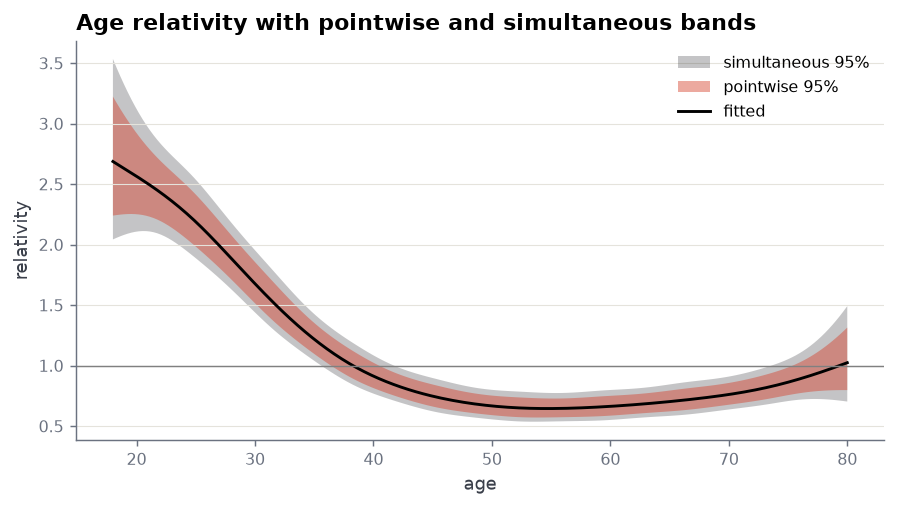
simultaneous_bands returns the same curve with both band types side by side.
Pointwise bands hold at each age separately; simultaneous bands hold jointly
across the whole curve, which is what you need before claiming the curve is
non-flat. They are wider for it — about half again as wide here. Drawn
together, the difference is the outer shaded band: even the simultaneous band
stays clear of the flat line at 1.0 below age 35 and again between the early
forties and the low seventies, so the shape survives the joint statement, not
only the pointwise one.
import matplotlib.pyplot as plt

bands = model.simultaneous_bands("age")
fig, ax = plt.subplots(figsize=(7, 4))
ax.fill_between(
    bands["x"],
    bands["ci_lower_simultaneous"],
    bands["ci_upper_simultaneous"],
    alpha=0.25,
    label="simultaneous 95%",
)
ax.fill_between(
    bands["x"],
    bands["ci_lower_pointwise"],
    bands["ci_upper_pointwise"],
    alpha=0.45,
    label="pointwise 95%",
)
ax.plot(bands["x"], bands["relativity"], color="black", linewidth=1.6, label="fitted")
ax.axhline(1.0, color="0.5", linewidth=0.8)
ax.set_xlabel("age")
ax.set_ylabel("relativity")
ax.set_title("Age relativity with pointwise and simultaneous bands")
ax.legend(loc="upper right")
fig.tight_layout()
drop1 refits without each feature and reports the deviance it cost;
term_importance scores the same features by the weighted variance of their
contribution to the linear predictor. They answer different questions —
significance against spread — and here they agree on the order: age first,
then region, then vehicle power.
effects = model.drop1(X, claims, offset=offset)[
    ["feature", "delta_deviance", "delta_df", "p_value"]
].merge(model.term_importance(X)[["feature", "sd_eta", "edf"]], on="feature")
effects["p_value"] = effects["p_value"].map("{:.1e}".format)
effects.round(3)
| feature | delta_deviance | delta_df | p_value | sd_eta | edf | |
|---|---|---|---|---|---|---|
| 0 | age | 325.956 | 4.577 | 1.0e-68 | 0.458 | 4.577 |
| 1 | region | 68.948 | 3.001 | 7.2e-15 | 0.239 | 3.000 |
| 2 | veh_power | 55.142 | 1.001 | 1.1e-13 | 0.210 | 1.000 |
metrics recomputes the fit statistics on any frame, so the same call gives
training numbers here and holdout numbers on a validation split. The fields are
plain attributes.
fit_metrics = model.metrics(X, claims, offset=offset)
pd.DataFrame(
    {
        "value": [
            fit_metrics.n_obs,
            fit_metrics.effective_df,
            fit_metrics.deviance,
            fit_metrics.explained_deviance,
            fit_metrics.log_likelihood,
            fit_metrics.aic,
            fit_metrics.bic,
        ]
    },
    index=[
        "n_obs",
        "effective_df",
        "deviance",
        "explained_deviance",
        "log_likelihood",
        "aic",
        "bic",
    ],
).round(3)
| value | |
|---|---|
| n_obs | 4000.000 |
| effective_df | 9.577 |
| deviance | 2983.765 |
| explained_deviance | 0.130 |
| log_likelihood | -2563.738 |
| aic | 5146.630 |
| bic | 5206.906 |